Вычисление частной производной python

Дифференцирование и интегрирование функций#

В рамказ компьютерной арифметики предельный переход осуществить невозможно, поэтому в целях аппроксимации производной нередко вместо предела при \(h \to 0\) подставляют очень малое \(h\) :

Такая аппроксимация производной называется правой разностной производной. Можно показать, что асимптотическая погрешность вычисления производной таким способом имеет вид \(o(h)\) , т.е. уменьшая шаг \(h\) можно добиться любой точности вычисления производной. Более распространенна центральная разнастная производная, определяемая выражением

Её асимптотическая погрешность имеет вид \(o(h^2)\) , а значит уменьшая шаг \(h\) в 2 раза, можно ожидать уменьшение погрешности вычисления производной в 4 раза.

Аналогичным образом можно определить аппроксимацию производной любого порядка. Метод scipy.misc.derivative в SciPy вычисляет разностную производную произвольного порядка (опциональный параметр n ).

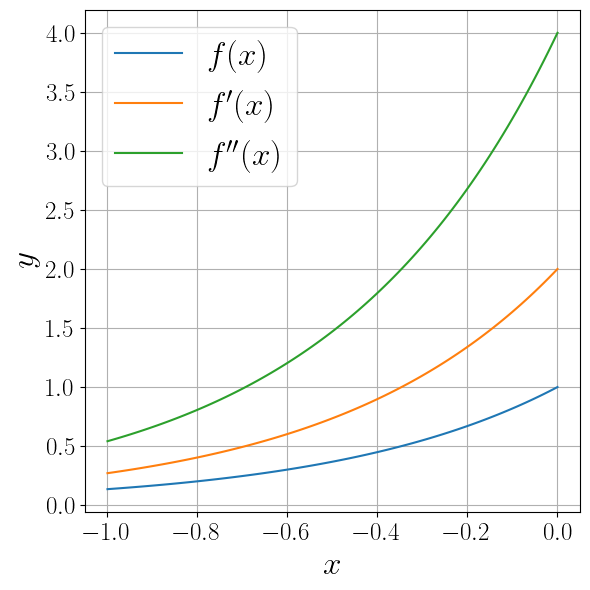
Продемонстрируем его применение на примере функции \(f(x) = e^\) .

from scipy.misc import derivative import numpy as np def f(x): return np.exp(2. * x) fig, ax = plt.subplots(figsize=(6, 6), layout="tight") x = np.linspace(-1, 0, 100) labels = ("$f(x)$", "$f'(x)$", "$f''(x)$") for n, label in enumerate(labels): y = derivative(f, x, n=n, dx=1e-3, order=2*n+1) if order > 0 else f(x) ax.plot(x, y, label=label) ax.set_xlabel("$x$") ax.set_ylabel("$y$") ax.legend() ax.grid() 

Аналитическое дифференцирование#

Ряд современных библиотек умеет вычислять производные от своих методов. Например, библиотека autograd.

Обратите внимание, что для аналитического вычисления производной средствами библиотеки autograd , необходимо вместо библиотеки NumPy использовать модуль autograd.numpy .

from autograd import numpy as np from autograd import elementwise_grad fig, ax = plt.subplots(figsize=(6, 6), layout="tight") x = np.linspace(-1, 0, 100) labels = ("$f(x)$", "$f'(x)$", "$f''(x)$") funcs = (f, elementwise_grad(f), elementwise_grad(elementwise_grad(f))) for order, (label, func) in enumerate(zip(labels, funcs)): ax.plot(x, func(x), label=label) ax.set_xlabel("$x$") ax.set_ylabel("$y$") ax.legend() ax.grid() 

Интегрирование функций#

Подмодуль scipy.integrate позволяет приближенно вычислять значение определенных интегралов.

Однократные интегралы#

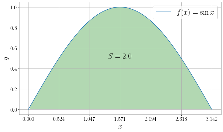
Функция scipy.integrate.quad позволяет проинтегрировать функцию \(f\colon \mathbb \to \mathbb\) . Вызов функции quad(f, a, b) приближенно находит значение интеграла

В качестве примера найдем численно значение интеграла

import numpy as np from scipy import integrate from matplotlib import pyplot as plt f = np.sin a, b = 0, np.pi I, _ = integrate.quad(f, 0, np.pi) x = np.linspace(0, np.pi, 100) y = f(x) fig, ax = plt.subplots(figsize=(10, 6), layout="tight") ax.plot(x, y, label=r"$f(x)=\sin x$") ax.set_xlabel("$x$") ax.set_ylabel("$y$") ax.fill_between(x, np.zeros_like(x), y, where=(y>0), facecolor='green', alpha=0.30) ax.set_xticks(np.linspace(0, np.pi, 7)) ax.text(np.pi/2, 0.5, fr"$S = I>$", fontdict="size": 24, "ha": "center">) ax.legend() ax.grid() 

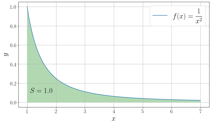
Параметры \(a\) и \(b\) могут принимать значения -inf и +inf , чтобы брать несобственные интегралы. Продемонстрируем это на примере интеграла

def f(x): return 1. / np.square(x) a, b = 1, np.inf I, _ = integrate.quad(f, a, b) x = np.linspace(a, 7, 100) y = f(x) fig, ax = plt.subplots(figsize=(10, 6), layout="tight") ax.plot(x, y, label=r"$f(x)=\dfrac $") ax.set_xlabel("$x$") ax.set_ylabel("$y$") ax.fill_between(x, np.zeros_like(x), y, where=(y>0), facecolor='green', alpha=0.30) ax.set_xticks(np.linspace(1, 7, 7)) ax.text(1.5, 0.1, fr"$S = I>$", fontdict="size": 24, "ha": "center">) ax.legend() ax.grid() 

Однако численное взятие несобственных интегралов отнюдь не тривиальная задача. Например, интеграл Френеля $ \( \int\limits_0^\infty \sin x^2 \, dx = \sqrt<\dfrac<\pi>> \) $

просто так вычислить не удастся.

def f(t): return np.sin(t**2) I, _ = integrate.quad(f, 0, np.inf) print(I) 

C:\Users\fadeev\AppData\Local\Temp/ipykernel_8252/3166585030.py:4: IntegrationWarning: The integral is probably divergent, or slowly convergent. I, _ = integrate.quad(f, 0, np.inf)

Интегралы большей кратности#

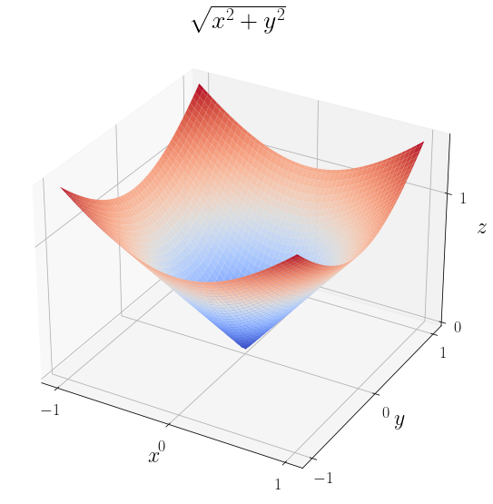
Функция scipy.integrate.dblquad позволяет вычислять интегралы вида

В качестве примера возьмём интеграл функции \(f = \sqrt\) в области \(D\) совпадающей с кругом единичного радиуса с центром в начале:

import numpy as np from scipy import integrate from matplotlib import pyplot as plt def h(x): return np.sqrt(1 - x**2) def g(x): return -h(x) def f(x, y): return np.sqrt(x**2 + y**2) a, b = -1, 1 I, _ = integrate.dblquad(f, -1, 1, g, h) x = np.linspace(a, b, 100) y = np.linspace(a, b, 100) x, y = np.meshgrid(x, y) z = f(x, y) fig, ax = plt.subplots(figsize=(8, 8), layout="tight", subplot_kw="projection": "3d">) ax.plot_surface(x, y, z, cmap="coolwarm") ax.set_xlabel("$x$") ax.set_ylabel("$y$") ax.set_zlabel("$z$") ax.set_xticks([-1, 0, 1]) ax.set_yticks([-1, 0, 1]) ax.set_zticks([0, 1]) ax.set_title(r"$\sqrt$") print(f"Вычисленное значение интеграла: I>, точное значение: 2*np.pi/3>.") 

Вычисленное значение интеграла: 2.0943951023924106, точное значение: 2.0943951023931953.

Трехкратные интегралы вида

можно вычислить методом integrate.tplquad. Интеграл произвольной кратности можно вычислить методом integrate.tplquad.

Источник

Вычисление производной

Для вычисления производных будем использовать библиотеку SymPy. Это библиотека с открытым исходным кодом, полностью написанная на языке Python. Разрабатывается как система компьютерной алгебры.

Подключение SymPy

Вначале нам необходимо установить библиотеку. Для этого в терминале (командной строке) следует ввести команду: pip install sympy .

Для подключения библиотеки в коде на Python 3 следует использовать ключевое слово import .

Чтобы не писать перед всеми функциями sympy с точкой, подключу следующим образом:

Следует обратить внимание, что в SymPy объявлено множество классов и функций, имена которых могут пересекаться с названиями в других библиотеках. Например, если используете библиотеку math, то там также есть sin , cos , pi и другие.

Формула российских дорог

Например, возьмем функцию с двумя независимыми переменными, типа поверхности y=f(x, z). Воспользуемся формулой российских дорог: y=sin(x)+0,5·z.

Перед тем как взять производную этой функции в Python, надо объявить все переменные, которые будут использоваться в ней. Для этого следует воспользоваться функцией symbols . В качестве аргумента используем строку с перечисленными через запятую или пробел названиями переменных.

После этого берем частную производную в Python 3 с помощью функции diff . Первым аргументом пишем функцию, вторым – переменную, по которой будем её дифференцировать.

Результат выводим с помощью print .

Дорога в горку

from sympy import * x, z = symbols('x z') print(diff(sin(x)+0.5*z, z)) 0.500000000000000

В результате получили 0.5. Частная производная по z положительна, следовательно, дорога в горку.

Дорога с колеёй

Теперь возьмём производную по x:

from sympy import * x, z = symbols('x z') print(diff(sin(x)+0.5*z, x)) cos(x)

Получили, что частная производная по x равна cos(x). Трактору на колею наплевать, ему важен только наклон горки.

В зависимости от задачи берем производную по нужному параметру.

В функции diff при необходимости, можно указать третьим параметром порядок дифференцирования. Так как мы вычисляли производную первого порядка, то его не указывали.

Источник

Derivatives in Python using SymPy

How to calculate derivatives in Python? In this article, we’ll use the Python SymPy library to play around with derivatives.

What are derivatives?

Derivatives are the fundamental tools of Calculus. It is very useful for optimizing a loss function with gradient descent in Machine Learning is possible only because of derivatives.

Suppose we have a function y = f(x) which is dependent on x then the derivation of this function means the rate at which the value y of the function changes with the change in x.

This is by no means an article about the fundamentals of derivatives, it can’t be. Calculus is a different beast that requires special attention. I presume you have some background in calculus. This article is intended to demonstrate how we can differentiate a function using the Sympy library.

Solving Derivatives in Python using SymPy

Python SymPy library is created for symbolic mathematics. The SymPy project aims to become a full-featured computer algebra system (CAS) while keeping the code simple to understand. Let’s see how to calculate derivatives in Python using SymPy.

1. Install SymPy using PIP

SymPy has more uses than just calculating derivatives but as of now, we’ll focus on derivatives. Let’s use PIP to install SymPy module.

2. Solving a differential with SymPy diff()

For differentiation, SymPy provides us with the diff method to output the derivative of the function.

Let’s see how can we achieve this using SymPy diff() function.

#Importing sympy from sympy import * # create a "symbol" called x x = Symbol('x') #Define function f = x**2 #Calculating Derivative derivative_f = f.diff(x) derivative_f

Declaring a symbol is similar to saying that our function has a variable ‘x’ or simply the function depends on x.

3. Solving Derivatives in Python

SymPy has lambdify function to calculate the derivative of the function that accepts symbol and the function as argument. Let’s look at example of calculating derivative using SymPy lambdify function.

from sympy import * # create a "symbol" called x x = Symbol('x') #Define function f = x**2 f1 = lambdify(x, f) #passing x=2 to the function f1(2)

Basic Derivative Rules in Python SymPy

There are certain rules we can use to calculate the derivative of differentiable functions.

Some of the most encountered rules are:

Let’s dive into how can we actually use sympy to calculate derivatives as implied by the general differentiation rules.

1. Power Rule

Example, Function we have : f(x) = x⁵

It’s derivative will be : f'(x) = 5x (5-1) = 5x 4

import sympy as sym #Power rule x = sym.Symbol('x') f = x**5 derivative_f = f.diff(x) derivative_f

2. Product Rule

Let u(x) and v(x) be differentiable functions. Then the product of the functions u(x)v(x) is also differentiable.

import sympy as sym #Product Rule x = sym.Symbol('x') f = sym.exp(x)*sym.cos(x) derivative_f = f.diff(x) derivative_f

3. Chain Rule

The chain rule calculate the derivative of a composition of functions.

• Say, we have a function h(x) = f( g(x) )
• Then according to chain rule: h′(x) = f ′(g(x)) g′(x)
• Example: f(x) = cos(x**2)

This process can be extended for quotient rule also. It must be obvious by now that only the function is changing while the application process remains the same, the remaining is taken care of by the library itself.

import sympy as sym #Chain Rule x = sym.Symbol('x') f = sym.cos(x**2) derivative_f = f.diff(x) derivative_f

Python Partial Derivative using SymPy

The examples we saw above just had one variable. But we are more likely to encounter functions having more than one variables. Such derivatives are generally referred to as partial derivative.

A partial derivative of a multivariable function is a derivative with respect to one variable with all other variables held constant.

Example: f(x,y) = x 4 + x * y 4

Let’s partially differentiate the above derivatives in Python w.r.t x.

import sympy as sym #Derivatives of multivariable function x , y = sym.symbols('x y') f = x**4+x*y**4 #Differentiating partially w.r.t x derivative_f = f.diff(x) derivative_f

We use symbols method when the number of variables is more than 1. Now, differentiate the derivatives in Python partially w.r.t y

import sympy as sym #Derivatives of multivariable function x , y = sym.symbols('x y') f = x**4+x*y**4 #Differentiating partially w.r.t y derivative_f = f.diff(y) derivative_f

The code is exactly similar but now y is passed as input argument in diff method.

We can choose to partially differentiate function first w.r.t x and then y.

import sympy as sym #Derivatives of multivariable function x , y = sym.symbols('x y') f = x**4+x*y**4 #Differentiating partially w.r.t x and y derivative_f = f.diff(x,y) derivative_f

Summary

This article by no means was a course about derivatives or how can we solve derivatives in Python but an article about how can we leverage python SymPy packages to perform differentiation on functions. Derivatives are awesome and you should definitely get the idea behind it as they play a crucial role in Machine learning and beyond.

What’s Next?

Resources

Источник