How to visualize a single Decision Tree from the Random Forest in Scikit-Learn (Python)?

The Random Forest is an esemble of Decision Trees. A single Decision Tree can be easily visualized in several different ways. In this post I will show you, how to visualize a Decision Tree from the Random Forest.
First let’s train Random Forest model on Boston data set (it is house price regression task available in scikit-learn ).
# Load packages import pandas as pd from sklearn.datasets import load_boston from sklearn.ensemble import RandomForestRegressor from sklearn import tree from dtreeviz.trees import dtreeviz # will be used for tree visualization from matplotlib import pyplot as plt plt.rcParams.update('figure.figsize': (12.0, 8.0)>) plt.rcParams.update('font.size': 14>) Load the data and train the Random Forest.
boston = load_boston() X = pd.DataFrame(boston.data, columns=boston.feature_names) y = boston.target Let’s set the number of trees in the forest to 100 (it is a default of n_estiamtors ):
rf = RandomForestRegressor(n_estimators=100) rf.fit(X, y) RandomForestRegressor(bootstrap=True, ccp_alpha=0.0, criterion='mse', max_depth=None, max_features='auto', max_leaf_nodes=None, max_samples=None, min_impurity_decrease=0.0, min_impurity_split=None, min_samples_leaf=1, min_samples_split=2, min_weight_fraction_leaf=0.0, n_estimators=100, n_jobs=None, oob_score=False, random_state=None, verbose=0, warm_start=False) Decision Trees are stored in a list in the estimators_ attribute in the rf model. We can check the length of the list, which should be equal to n_estiamtors value.
We can plot a first Decision Tree from the Random Forest (with index 0 in the list):
plt.figure(figsize=(20,20)) _ = tree.plot_tree(rf.estimators_[0], feature_names=X.columns, filled=True) 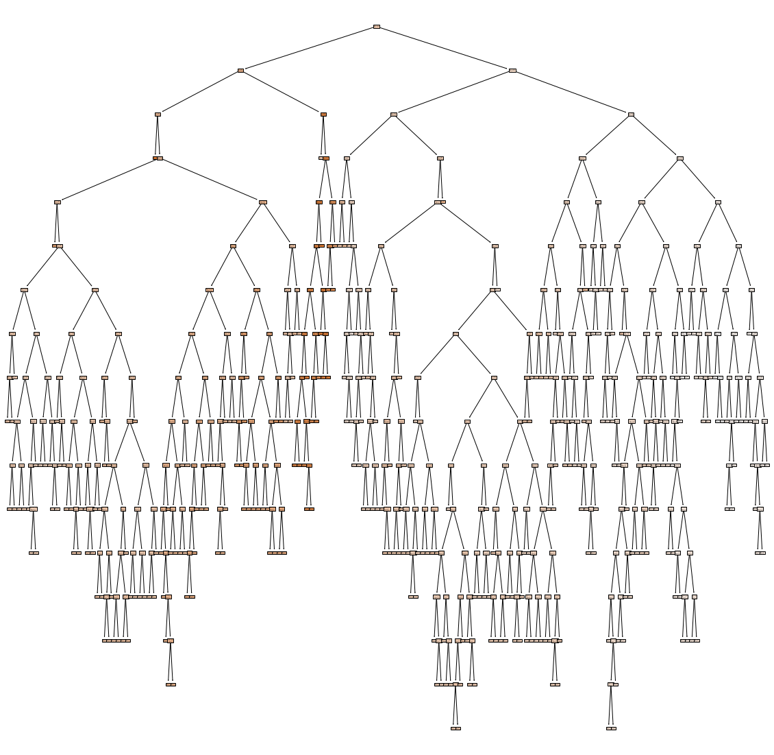
Do you understand anything? The tree is too large to visualize it in one figure and make it readable.
Let’s check the depth of the first tree from the Random Forest:
rf.estimators_[0].tree_.max_depth >>> 16 Our first tree has max_depth=16 . Other trees have similar depth. To make visualization readable it will be good to limit the depth of the tree. In MLJAR’s open-source AutoML package mljar-supervised the Decision Tree’s depth is set to be in range from 1 to 4. Let’s train the Random Forest again with max_depth=3 .
rf = RandomForestRegressor(n_estimators=100, max_depth=3) rf.fit(X, y) RandomForestRegressor(bootstrap=True, ccp_alpha=0.0, criterion='mse', max_depth=3, max_features='auto', max_leaf_nodes=None, max_samples=None, min_impurity_decrease=0.0, min_impurity_split=None, min_samples_leaf=1, min_samples_split=2, min_weight_fraction_leaf=0.0, n_estimators=100, n_jobs=None, oob_score=False, random_state=None, verbose=0, warm_start=False) The plot of first Decision Tree:
_ = tree.plot_tree(rf.estimators_[0], feature_names=X.columns, filled=True) 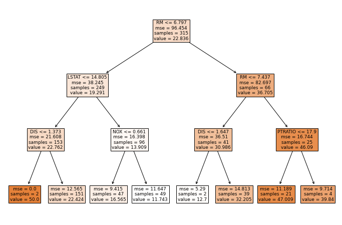
We can use dtreeviz package to visualize the first Decision Tree:
viz = dtreeviz(rf.estimators_[0], X, y, feature_names=X.columns, target_name="Target") viz Summary
I show you how to visualize the single Decision Tree from the Random Forest. Trees can be accessed by integer index from estimators_ list. Sometimes when the tree is too deep, it is worth to limit the depth of the tree with max_depth hyper-parameter. What is interesting, limiting the depth of the trees in the Random Forest will make the final model much smaller in terms of used RAM memory and disk space needed to save the model. It will also change the performance of the default Random Forest (with full trees), it will help or not, depending on the data set.
sklearn.tree .plot_tree
sklearn.tree. plot_tree ( decision_tree , * , max_depth = None , feature_names = None , class_names = None , label = ‘all’ , filled = False , impurity = True , node_ids = False , proportion = False , rounded = False , precision = 3 , ax = None , fontsize = None ) [source] 
The sample counts that are shown are weighted with any sample_weights that might be present.
The visualization is fit automatically to the size of the axis. Use the figsize or dpi arguments of plt.figure to control the size of the rendering.
The decision tree to be plotted.
max_depth int, default=None
The maximum depth of the representation. If None, the tree is fully generated.
feature_names list of str, default=None
Names of each of the features. If None, generic names will be used (“x[0]”, “x[1]”, …).
class_names list of str or bool, default=None
Names of each of the target classes in ascending numerical order. Only relevant for classification and not supported for multi-output. If True , shows a symbolic representation of the class name.
label , default=’all’
Whether to show informative labels for impurity, etc. Options include ‘all’ to show at every node, ‘root’ to show only at the top root node, or ‘none’ to not show at any node.
filled bool, default=False
When set to True , paint nodes to indicate majority class for classification, extremity of values for regression, or purity of node for multi-output.
impurity bool, default=True
When set to True , show the impurity at each node.
node_ids bool, default=False
When set to True , show the ID number on each node.
proportion bool, default=False
When set to True , change the display of ‘values’ and/or ‘samples’ to be proportions and percentages respectively.
rounded bool, default=False
When set to True , draw node boxes with rounded corners and use Helvetica fonts instead of Times-Roman.
precision int, default=3
Number of digits of precision for floating point in the values of impurity, threshold and value attributes of each node.
ax matplotlib axis, default=None
Axes to plot to. If None, use current axis. Any previous content is cleared.
fontsize int, default=None
Size of text font. If None, determined automatically to fit figure.
Returns : annotations list of artists
List containing the artists for the annotation boxes making up the tree.
>>> from sklearn.datasets import load_iris >>> from sklearn import tree
>>> clf = tree.DecisionTreeClassifier(random_state=0) >>> iris = load_iris()
>>> clf = clf.fit(iris.data, iris.target) >>> tree.plot_tree(clf) [. ]