scipy.stats.chisquare#
The chi-square test tests the null hypothesis that the categorical data has the given frequencies.
Parameters : f_obs array_like
Observed frequencies in each category.
f_exp array_like, optional
Expected frequencies in each category. By default the categories are assumed to be equally likely.
ddof int, optional
“Delta degrees of freedom”: adjustment to the degrees of freedom for the p-value. The p-value is computed using a chi-squared distribution with k — 1 — ddof degrees of freedom, where k is the number of observed frequencies. The default value of ddof is 0.
axis int or None, optional
The axis of the broadcast result of f_obs and f_exp along which to apply the test. If axis is None, all values in f_obs are treated as a single data set. Default is 0.
Returns : res: Power_divergenceResult
An object containing attributes:
The chi-squared test statistic. The value is a float if axis is None or f_obs and f_exp are 1-D.
The p-value of the test. The value is a float if ddof and the return value chisq are scalars.
Fisher exact test on a 2×2 contingency table.
An unconditional exact test. An alternative to chi-squared test for small sample sizes.
This test is invalid when the observed or expected frequencies in each category are too small. A typical rule is that all of the observed and expected frequencies should be at least 5. According to [3], the total number of samples is recommended to be greater than 13, otherwise exact tests (such as Barnard’s Exact test) should be used because they do not overreject.
Also, the sum of the observed and expected frequencies must be the same for the test to be valid; chisquare raises an error if the sums do not agree within a relative tolerance of 1e-8 .
The default degrees of freedom, k-1, are for the case when no parameters of the distribution are estimated. If p parameters are estimated by efficient maximum likelihood then the correct degrees of freedom are k-1-p. If the parameters are estimated in a different way, then the dof can be between k-1-p and k-1. However, it is also possible that the asymptotic distribution is not chi-square, in which case this test is not appropriate.
Pearson, Karl. “On the criterion that a given system of deviations from the probable in the case of a correlated system of variables is such that it can be reasonably supposed to have arisen from random sampling”, Philosophical Magazine. Series 5. 50 (1900), pp. 157-175.
Mannan, R. William and E. Charles. Meslow. “Bird populations and vegetation characteristics in managed and old-growth forests, northeastern Oregon.” Journal of Wildlife Management 48, 1219-1238, DOI:10.2307/3801783, 1984.
In [4], bird foraging behavior was investigated in an old-growth forest of Oregon. In the forest, 44% of the canopy volume was Douglas fir, 24% was ponderosa pine, 29% was grand fir, and 3% was western larch. The authors observed the behavior of several species of birds, one of which was the red-breasted nuthatch. They made 189 observations of this species foraging, recording 43 (“23%”) of observations in Douglas fir, 52 (“28%”) in ponderosa pine, 54 (“29%”) in grand fir, and 40 (“21%”) in western larch.
Using a chi-square test, we can test the null hypothesis that the proportions of foraging events are equal to the proportions of canopy volume. The authors of the paper considered a p-value less than 1% to be significant.
Using the above proportions of canopy volume and observed events, we can infer expected frequencies.
>>> import numpy as np >>> f_exp = np.array([44, 24, 29, 3]) / 100 * 189
The observed frequencies of foraging were:
>>> f_obs = np.array([43, 52, 54, 40])
We can now compare the observed frequencies with the expected frequencies.
>>> from scipy.stats import chisquare >>> chisquare(f_obs=f_obs, f_exp=f_exp) Power_divergenceResult(statistic=228.23515947653874, pvalue=3.3295585338846486e-49)
The p-value is well below the chosen significance level. Hence, the authors considered the difference to be significant and concluded that the relative proportions of foraging events were not the same as the relative proportions of tree canopy volume.
Following are other generic examples to demonstrate how the other parameters can be used.
When just f_obs is given, it is assumed that the expected frequencies are uniform and given by the mean of the observed frequencies.
>>> chisquare([16, 18, 16, 14, 12, 12]) Power_divergenceResult(statistic=2.0, pvalue=0.84914503608460956)
With f_exp the expected frequencies can be given.
>>> chisquare([16, 18, 16, 14, 12, 12], f_exp=[16, 16, 16, 16, 16, 8]) Power_divergenceResult(statistic=3.5, pvalue=0.62338762774958223)
When f_obs is 2-D, by default the test is applied to each column.
>>> obs = np.array([[16, 18, 16, 14, 12, 12], [32, 24, 16, 28, 20, 24]]).T >>> obs.shape (6, 2) >>> chisquare(obs) Power_divergenceResult(statistic=array([2. , 6.66666667]), pvalue=array([0.84914504, 0.24663415]))
By setting axis=None , the test is applied to all data in the array, which is equivalent to applying the test to the flattened array.
>>> chisquare(obs, axis=None) Power_divergenceResult(statistic=23.31034482758621, pvalue=0.015975692534127565) >>> chisquare(obs.ravel()) Power_divergenceResult(statistic=23.310344827586206, pvalue=0.01597569253412758)
ddof is the change to make to the default degrees of freedom.
>>> chisquare([16, 18, 16, 14, 12, 12], ddof=1) Power_divergenceResult(statistic=2.0, pvalue=0.7357588823428847)
The calculation of the p-values is done by broadcasting the chi-squared statistic with ddof.
>>> chisquare([16, 18, 16, 14, 12, 12], ddof=[0,1,2]) Power_divergenceResult(statistic=2.0, pvalue=array([0.84914504, 0.73575888, 0.5724067 ]))
f_obs and f_exp are also broadcast. In the following, f_obs has shape (6,) and f_exp has shape (2, 6), so the result of broadcasting f_obs and f_exp has shape (2, 6). To compute the desired chi-squared statistics, we use axis=1 :
>>> chisquare([16, 18, 16, 14, 12, 12], . f_exp=[[16, 16, 16, 16, 16, 8], [8, 20, 20, 16, 12, 12]], . axis=1) Power_divergenceResult(statistic=array([3.5 , 9.25]), pvalue=array([0.62338763, 0.09949846]))
scipy.stats.chi2#
For the noncentral chi-square distribution, see ncx2 .
As an instance of the rv_continuous class, chi2 object inherits from it a collection of generic methods (see below for the full list), and completes them with details specific for this particular distribution.
The probability density function for chi2 is:
for \(x > 0\) and \(k > 0\) (degrees of freedom, denoted df in the implementation).
chi2 takes df as a shape parameter.
The chi-squared distribution is a special case of the gamma distribution, with gamma parameters a = df/2 , loc = 0 and scale = 2 .
The probability density above is defined in the “standardized” form. To shift and/or scale the distribution use the loc and scale parameters. Specifically, chi2.pdf(x, df, loc, scale) is identically equivalent to chi2.pdf(y, df) / scale with y = (x — loc) / scale . Note that shifting the location of a distribution does not make it a “noncentral” distribution; noncentral generalizations of some distributions are available in separate classes.
>>> import numpy as np >>> from scipy.stats import chi2 >>> import matplotlib.pyplot as plt >>> fig, ax = plt.subplots(1, 1)
Calculate the first four moments:
>>> df = 55 >>> mean, var, skew, kurt = chi2.stats(df, moments='mvsk')
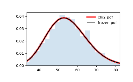
Display the probability density function ( pdf ):
>>> x = np.linspace(chi2.ppf(0.01, df), . chi2.ppf(0.99, df), 100) >>> ax.plot(x, chi2.pdf(x, df), . 'r-', lw=5, alpha=0.6, label='chi2 pdf')
Alternatively, the distribution object can be called (as a function) to fix the shape, location and scale parameters. This returns a “frozen” RV object holding the given parameters fixed.
Freeze the distribution and display the frozen pdf :
>>> rv = chi2(df) >>> ax.plot(x, rv.pdf(x), 'k-', lw=2, label='frozen pdf')
Check accuracy of cdf and ppf :
>>> vals = chi2.ppf([0.001, 0.5, 0.999], df) >>> np.allclose([0.001, 0.5, 0.999], chi2.cdf(vals, df)) True
And compare the histogram:
>>> ax.hist(r, density=True, bins='auto', histtype='stepfilled', alpha=0.2) >>> ax.set_xlim([x[0], x[-1]]) >>> ax.legend(loc='best', frameon=False) >>> plt.show()
rvs(df, loc=0, scale=1, size=1, random_state=None)
pdf(x, df, loc=0, scale=1)
Probability density function.
logpdf(x, df, loc=0, scale=1)
Log of the probability density function.
cdf(x, df, loc=0, scale=1)
Cumulative distribution function.
logcdf(x, df, loc=0, scale=1)
Log of the cumulative distribution function.
sf(x, df, loc=0, scale=1)
Survival function (also defined as 1 — cdf , but sf is sometimes more accurate).
logsf(x, df, loc=0, scale=1)
Log of the survival function.
ppf(q, df, loc=0, scale=1)
Percent point function (inverse of cdf — percentiles).
isf(q, df, loc=0, scale=1)
Inverse survival function (inverse of sf ).
moment(order, df, loc=0, scale=1)
Non-central moment of the specified order.
stats(df, loc=0, scale=1, moments=’mv’)
Mean(‘m’), variance(‘v’), skew(‘s’), and/or kurtosis(‘k’).
entropy(df, loc=0, scale=1)
(Differential) entropy of the RV.
Parameter estimates for generic data. See scipy.stats.rv_continuous.fit for detailed documentation of the keyword arguments.
expect(func, args=(df,), loc=0, scale=1, lb=None, ub=None, conditional=False, **kwds)
Expected value of a function (of one argument) with respect to the distribution.
median(df, loc=0, scale=1)
Median of the distribution.
mean(df, loc=0, scale=1)
var(df, loc=0, scale=1)
Variance of the distribution.
std(df, loc=0, scale=1)
Standard deviation of the distribution.
interval(confidence, df, loc=0, scale=1)
Confidence interval with equal areas around the median.
Как выполнить тест на соответствие хи-квадрат в Python
Хи-квадрат критерий согласия используется для определения того, следует ли категориальная переменная гипотетическому распределению.
В этом учебном пособии объясняется, как выполнить критерий согласия Хи-квадрат в Python.
Пример: критерий согласия хи-квадрат в Python
Владелец магазина утверждает, что каждый будний день в его магазин приходит одинаковое количество покупателей. Чтобы проверить эту гипотезу, исследователь записывает количество покупателей, которые заходят в магазин на данной неделе, и обнаруживает следующее:
Используйте следующие шаги, чтобы выполнить тест на соответствие хи-квадрат в Python, чтобы определить, согласуются ли данные с заявлением владельца магазина.
Шаг 1: Создайте данные.
Во-первых, мы создадим два массива для хранения наблюдаемого и ожидаемого количества клиентов на каждый день:
expected = [50, 50, 50, 50, 50] observed = [50, 60, 40, 47, 53] Шаг 2: Проведите тест на соответствие хи-квадрату.
Затем мы можем выполнить критерий согласия Хи-квадрат с помощью функции хи-квадрат из библиотеки SciPy, которая использует следующий синтаксис:
хи-квадрат (f_obs, f_exp)
- f_obs: массив наблюдаемых счетчиков.
- f_exp: массив ожидаемых значений. По умолчанию предполагается, что каждая категория равновероятна.
Следующий код показывает, как использовать эту функцию в нашем конкретном примере:
import scipy.stats as stats #perform Chi-Square Goodness of Fit Test stats.chisquare(f_obs=observed, f_exp=expected) (statistic=4.36, pvalue=0.35947) Статистический показатель теста хи-квадрат равен 4,36 , а соответствующее значение p равно 0,35947 .
Обратите внимание, что значение p соответствует значению хи-квадрата с n-1 степенями свободы (степеней свободы), где n — количество различных категорий. В этом случае степень свободы = 5-1 = 4. Вы можете использовать Калькулятор значений хи-квадрат для P , чтобы убедиться, что значение p, соответствующее X 2 = 4,36 при степени свободы = 4, равно 0,35947 .
Напомним, что критерий согласия Хи-квадрат использует следующие нулевую и альтернативную гипотезы:
- H 0 : (нулевая гипотеза) Переменная следует за гипотетическим распределением.
- H 1 : (альтернативная гипотеза) Переменная не подчиняется предполагаемому распределению.
Поскольку p-значение (0,35947) не меньше 0,05, мы не можем отвергнуть нулевую гипотезу. Это означает, что у нас нет достаточных доказательств того, что истинное распределение покупателей отличается от распределения, о котором заявил владелец магазина.