Short time fourier transform python
The Short Time Fourier Transform (STFT) is a special flavor of a Fourier transform where you can see how your frequencies in your signal change through time. It works by slicing up your signal into many small segments and taking the fourier transform of each of these. The result is usually a waterfall plot which shows frequency against time. I’ll talk more in depth about the STFT in a later post, for now let’s focus on the code.
I was looking for a way to do STFT’s using Numpy, but to my chagrin it looks like there isn’t an easy function implemented. Well then, I’ll just write my own.
First, let’s look at the desired result that I’m trying to obtain. Here is a spectrum of a whistle performed by my friend Mike.
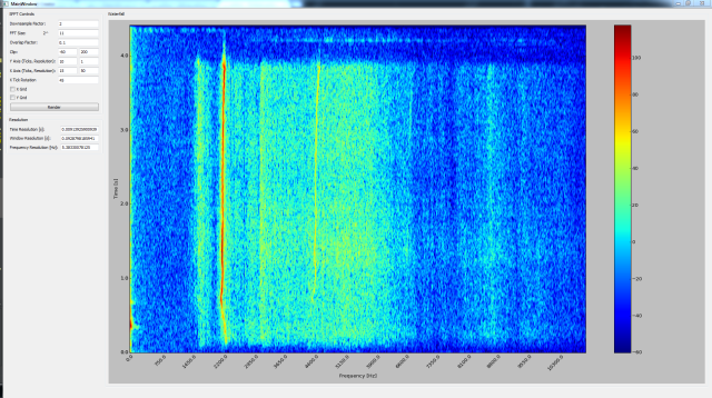
You can see that there is a strong frequency around 2200 Hz which makes this note about a C# or Dd in the 7th octave. Mike The second harmonic is also fairly strong at 4400 Hz.
Here is a picture of a whistle which increases in frequency over time.
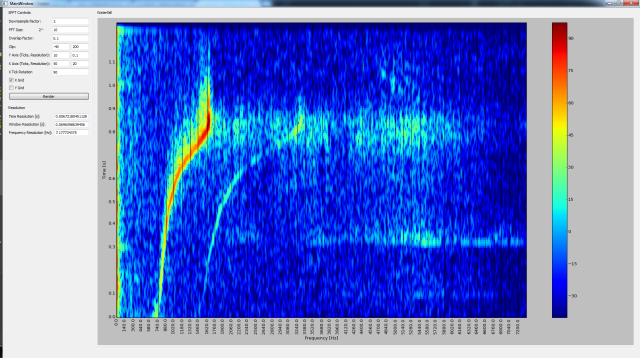
Spectrum of a chirp like whistle
It goes from 880 Hz (A in the 5th octave) all the way up to 1760 Hz (A in the 6th octave). I find it remarkable how precisely Mike managed to whistle an octave as he wasn’t trying to do that…
STFT Algorithm:
So, we understand what we’re trying to make – now we have to figure out how to make it. The data flow we have to achieve is pretty simple, as we only need to do the following steps:
- Pick out a short segment of data from the overall signal
- Multiply that segment against a half-cosine function
- Pad the end of the segment with zeros
- Take the Fourier transform of that segment and normalize it into positive and negative frequencies
- Combine the energy from the positive and negative frequencies together, and display the one-sided spectrum
- Scale the resulting spectrum into dB for easier viewing
- Clip the signal to remove noise past the noise floor which we don’t care about
Step 1 – Pick segment: We need to find our current segment to process from the overall data set. We use the concept of a ‘sliding window’ to help us visualize what’s happening. The data inside the window is the current segment to be processed.

Sliding window on top of data
The window’s length remains the same during the processing of the data, but the offset changes with each step of the algorithm. Usually when processing the STFT, the change in offset will be less than one window length, meaning that the last window and the current window overlap. If we define the window size, and the percentage of overlap, we know all the information we need about how the window moves throughout the processing.
Step 2 – Multiply by half-cosine: This helps to alleviate a problem created by segmenting the data. When the data is cut into pieces, the edges make a sharp transition that didn’t exist before. Multiplying by a half cosine function helps to fade the signal in and out so that the transitions at the edges do not affect the Fourier transform of the data.
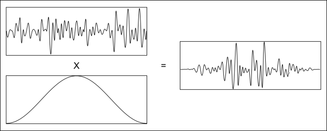
Data multiplied by a half cosine
There is an additional benefit to using a half cosine window. It can be shown that with an overlap factor of 50%, the sum of the windows is a constant value of 1. This means that multiplying our data by this particular function does not introduce differences in amplitude from the original signal. This is mostly important if the waveform has some type of units attached to it [pascals] and we want the frequencies in the Fourier transform to correctly represent the energy content of each frequency in those units.
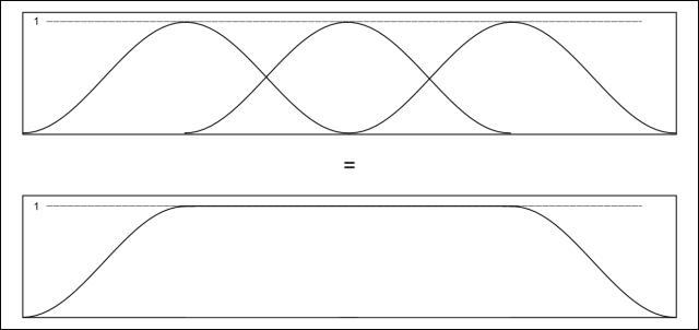
Half cosine windows combining into a unity gain.
Step 3 – Pad Data: We pad the end of the current segment with a number of zeros equal to the length of the window. Or in other words, the new segment will be twice as long as the original segment. The reason for this is explained later.
Step 4 – Fourier Transform and Scale: This is where all the magic happens. Everything up to this point was just preparing the data, but this step is the beating heart of the algorithm. Here we finally take the Fourier transform of the data. I’m not going to explain the Fourier transform here except to say that it takes a signal and extracts the frequency content from that signal. There are a few other things that need to be remembered about the Fourier transform.
- The number of samples of data in is equal to the number of frequency bins out
- The maximum frequency that can be represented is the Nyquist frequency, or half the sampling frequency of the data.
- In the the Discrete Fourier Transform (what we are using) the order of the frequency bins is 0 Hz (DC component), positive frequencies, Nyquist Frequency, negative frequencies
- The data from the Fourier transform needs to be scaled by the number of samples in the transform to maintain equal energy (according to Parseval’s theorem)
Step 5 – Autopower: This is just more post processing to make the results more palatable to look at. We find the autopower spectrum from the results of the Fourier transform. The autopower spectrum is a one-sided spectrum (only contains positive frequencies) as opposed to the two-sided spectrum returned by the Fourier transform – so it’s more like the actual real world which does not contain negative frequencies. The autopower spectrum is also scaled to represent the energy content that was in both the positive and negative frequencies of the Fourier transform. This is important for the ‘correctness’ of the energy content of each frequency, but also has the handy benefit of suppressing lower energy content and dramatizing higher energy content. Usually people only care about the higher energy content, so finding this transform typically makes the data much easier to look at.
Part of taking the autopwer spectrum is throwing away the upper half of the array of data. This is why we padded the segment to twice it’s size – so that when the result was cut down by half by the autopower transform, we would still have the same number of frequency bins as samples in our segment. Note that this isn’t a strict requirement of the algorithm – to have the segment size as frequency bins. We could have chosen our pad length to be any number from zero (no padding) to infinity. There is a trade off here which is too heavy in theory to go into fully here, suffice to say that I found this decision works well and simplifies the math.
Step 6 – Convert to DB: This is another transform to make the data easier to look at. It turns out that peoples ears work on a logarithmic scale so that the ear can detect much finer changes in amplitude at low amplitudes than at high amplitudes. We transform the data into decibels (dB) which is a logarithmic scale, so that we can see the energy content of a signal more how our ears would detect it. Converting the data to decibels has the effect of stretching peaks downwards towards the average sound level, and bringing troughs upwards. This allows us to compare content at all amplitude levels. If we didn’t do this and we scaled the data so that the peaks were visible, it would be impossible to see any shape in the quieter values, vs if we looked at the quieter values, the peaks would explode off the top of the screen.
Step 7 – Clip Data: This also makes the data easier to look at. We know from experience that everything below -40 dB is well below the noise floor and is probably just numerical error in the algorithm. Therefore, we can clip the data so that everything below -40 dB is set to -40 dB exactly. This gives us more color range to apply to significant portions of our data.
Here’s what the code looks like:
# data = a numpy array containing the signal to be processed # fs = a scalar which is the sampling frequency of the data hop_size = np.int32(np.floor(fft_size * (1-overlap_fac))) pad_end_size = fft_size # the last segment can overlap the end of the data array by no more than one window size total_segments = np.int32(np.ceil(len(data) / np.float32(hop_size))) t_max = len(data) / np.float32(fs) window = np.hanning(fft_size) # our half cosine window inner_pad = np.zeros(fft_size) # the zeros which will be used to double each segment size proc = np.concatenate((data, np.zeros(pad_end_size))) # the data to process result = np.empty((total_segments, fft_size), dtype=np.float32) # space to hold the result for i in xrange(total_segments): # for each segment current_hop = hop_size * i # figure out the current segment offset segment = proc[current_hop:current_hop+fft_size] # get the current segment windowed = segment * window # multiply by the half cosine function padded = np.append(windowed, inner_pad) # add 0s to double the length of the data spectrum = np.fft.fft(padded) / fft_size # take the Fourier Transform and scale by the number of samples autopower = np.abs(spectrum * np.conj(spectrum)) # find the autopower spectrum result[i, :] = autopower[:fft_size] # append to the results array result = 20*np.log10(result) # scale to db result = np.clip(result, -40, 200) # clip values
Displaying the Data:
Once we’ve completed the processing, we need to display our results on screen. This is pretty easy actually – the algorithm returns a 2D array of data with values ranging from -40 to our maximum value. One axis of the array represent frequency bins, and the other represents the segment number that was processed to get the frequency data.
Using matplotlib, we can simply display this array as an image. We’ll apply a color map so that -40 is dark blue, and our signal maximum is red and let matplotlib do all the heavy lifting to scale and interpolate our array to the size of our image, and then display it on screen.
We have to do some math to figure out what frequency each column in the array represents and what point in time each row represents, but after we have that, we can make tick marks and take a look at our data.
img = plt.imshow(result, origin='lower', cmap='jet', interpolation='nearest', aspect='auto') plt.show()
There is more code for making the GUI shown in the images above which will be posted soon.
Saved searches
Use saved searches to filter your results more quickly
You signed in with another tab or window. Reload to refresh your session. You signed out in another tab or window. Reload to refresh your session. You switched accounts on another tab or window. Reload to refresh your session.
Short-time Fourier transform in Python.
License
aluchies/stft
This commit does not belong to any branch on this repository, and may belong to a fork outside of the repository.
Name already in use
A tag already exists with the provided branch name. Many Git commands accept both tag and branch names, so creating this branch may cause unexpected behavior. Are you sure you want to create this branch?
Sign In Required
Please sign in to use Codespaces.
Launching GitHub Desktop
If nothing happens, download GitHub Desktop and try again.
Launching GitHub Desktop
If nothing happens, download GitHub Desktop and try again.
Launching Xcode
If nothing happens, download Xcode and try again.
Launching Visual Studio Code
Your codespace will open once ready.
There was a problem preparing your codespace, please try again.
Latest commit
Git stats
Files
Failed to load latest commit information.
README.md
Short-time Fourier transform (STFT) and inverse short-time Fourier transform (ISTFT) in python.
This module is based on the algorithm proposed in [1]. The features of this module include
- the input data is assumed to be real (use rfft/irfft instead of fft/ifft)
- it can be applied to an n-d array
- the segmentation is always along the first dimension
- overlapping segments are allowed
- zero padding is allowed
- the ISTFT can be performed using overlap-and-add (p=1) or a least squares approach (p=2).
- This module can be dropped into your project. Scipy also includes an stft/istft implementation.
Additional works that use this stft/istft approach include 3.
If you use this code in work that you publish, please consider citing at least one of 2.
[1] B Yang, «A study of inverse short-time Fourier transform,» in Proc. of ICASSP, 2008. [2] B Byram et al, «Ultrasonic multipath and beamforming clutter reduction: a chirp model approach,» IEEE UFFC, 61, 3, 2014. [3] B Byram et al, «A model and regularization scheme for ultrasonic beamforming clutter reduction, » IEEE UFFC, 62, 11, 2015. [4] A Luchies and B Byram, «Deep neural networks for ultrasound beamforming,» IEEE TMI, 37, 9, 2018. [5] A Luchies and B Byram, «Training improvements for ultrasound beamforming with deep neural networks,» PMB, 64, 4, 2019.About
Short-time Fourier transform in Python.