scipy.integrate.odeint#
scipy.integrate. odeint ( func , y0 , t , args = () , Dfun = None , col_deriv = 0 , full_output = 0 , ml = None , mu = None , rtol = None , atol = None , tcrit = None , h0 = 0.0 , hmax = 0.0 , hmin = 0.0 , ixpr = 0 , mxstep = 0 , mxhnil = 0 , mxordn = 12 , mxords = 5 , printmessg = 0 , tfirst = False ) [source] #
Integrate a system of ordinary differential equations.
For new code, use scipy.integrate.solve_ivp to solve a differential equation.
Solve a system of ordinary differential equations using lsoda from the FORTRAN library odepack.
Solves the initial value problem for stiff or non-stiff systems of first order ode-s:
dy/dt = func(y, t, . ) [or func(t, y, . )]
By default, the required order of the first two arguments of func are in the opposite order of the arguments in the system definition function used by the scipy.integrate.ode class and the function scipy.integrate.solve_ivp . To use a function with the signature func(t, y, . ) , the argument tfirst must be set to True .
Computes the derivative of y at t. If the signature is callable(t, y, . ) , then the argument tfirst must be set True .
Initial condition on y (can be a vector).
A sequence of time points for which to solve for y. The initial value point should be the first element of this sequence. This sequence must be monotonically increasing or monotonically decreasing; repeated values are allowed.
args tuple, optional
Extra arguments to pass to function.
Dfun callable(y, t, …) or callable(t, y, …)
Gradient (Jacobian) of func. If the signature is callable(t, y, . ) , then the argument tfirst must be set True .
col_deriv bool, optional
True if Dfun defines derivatives down columns (faster), otherwise Dfun should define derivatives across rows.
full_output bool, optional
True if to return a dictionary of optional outputs as the second output
printmessg bool, optional
Whether to print the convergence message
tfirst bool, optional
If True, the first two arguments of func (and Dfun, if given) must t, y instead of the default y, t .
Array containing the value of y for each desired time in t, with the initial value y0 in the first row.
infodict dict, only returned if full_output == True
Dictionary containing additional output information
vector of step sizes successfully used for each time step
vector with the value of t reached for each time step (will always be at least as large as the input times)
vector of tolerance scale factors, greater than 1.0, computed when a request for too much accuracy was detected
value of t at the time of the last method switch (given for each time step)
cumulative number of time steps
cumulative number of function evaluations for each time step
cumulative number of jacobian evaluations for each time step
a vector of method orders for each successful step
index of the component of largest magnitude in the weighted local error vector (e / ewt) on an error return, -1 otherwise
the length of the double work array required
the length of integer work array required
a vector of method indicators for each successful time step: 1: adams (nonstiff), 2: bdf (stiff)
If either of these are not None or non-negative, then the Jacobian is assumed to be banded. These give the number of lower and upper non-zero diagonals in this banded matrix. For the banded case, Dfun should return a matrix whose rows contain the non-zero bands (starting with the lowest diagonal). Thus, the return matrix jac from Dfun should have shape (ml + mu + 1, len(y0)) when ml >=0 or mu >=0 . The data in jac must be stored such that jac[i — j + mu, j] holds the derivative of the i`th equation with respect to the `j`th state variable. If `col_deriv is True, the transpose of this jac must be returned.
rtol, atol float, optional
The input parameters rtol and atol determine the error control performed by the solver. The solver will control the vector, e, of estimated local errors in y, according to an inequality of the form max-norm of (e / ewt)
tcrit ndarray, optional
Vector of critical points (e.g., singularities) where integration care should be taken.
h0 float, (0: solver-determined), optional
The step size to be attempted on the first step.
hmax float, (0: solver-determined), optional
The maximum absolute step size allowed.
hmin float, (0: solver-determined), optional
The minimum absolute step size allowed.
ixpr bool, optional
Whether to generate extra printing at method switches.
mxstep int, (0: solver-determined), optional
Maximum number of (internally defined) steps allowed for each integration point in t.
mxhnil int, (0: solver-determined), optional
Maximum number of messages printed.
mxordn int, (0: solver-determined), optional
Maximum order to be allowed for the non-stiff (Adams) method.
mxords int, (0: solver-determined), optional
Maximum order to be allowed for the stiff (BDF) method.
solve an initial value problem for a system of ODEs
a more object-oriented integrator based on VODE
for finding the area under a curve
The second order differential equation for the angle theta of a pendulum acted on by gravity with friction can be written:
theta''(t) + b*theta'(t) + c*sin(theta(t)) = 0
where b and c are positive constants, and a prime (’) denotes a derivative. To solve this equation with odeint , we must first convert it to a system of first order equations. By defining the angular velocity omega(t) = theta'(t) , we obtain the system:
theta'(t) = omega(t) omega'(t) = -b*omega(t) - c*sin(theta(t))
Let y be the vector [theta, omega]. We implement this system in Python as:
>>> import numpy as np >>> def pend(y, t, b, c): . theta, omega = y . dydt = [omega, -b*omega - c*np.sin(theta)] . return dydt .
We assume the constants are b = 0.25 and c = 5.0:
For initial conditions, we assume the pendulum is nearly vertical with theta(0) = pi — 0.1, and is initially at rest, so omega(0) = 0. Then the vector of initial conditions is
We will generate a solution at 101 evenly spaced samples in the interval 0 t
Call odeint to generate the solution. To pass the parameters b and c to pend, we give them to odeint using the args argument.
>>> from scipy.integrate import odeint >>> sol = odeint(pend, y0, t, args=(b, c))
The solution is an array with shape (101, 2). The first column is theta(t), and the second is omega(t). The following code plots both components.
>>> import matplotlib.pyplot as plt >>> plt.plot(t, sol[:, 0], 'b', label='theta(t)') >>> plt.plot(t, sol[:, 1], 'g', label='omega(t)') >>> plt.legend(loc='best') >>> plt.xlabel('t') >>> plt.grid() >>> plt.show()
Dynamics and Control
Differential equations are solved in Python with the Scipy.integrate package using function odeint or solve_ivp.

Jupyter Notebook ODEINT Examples on GitHub

Jupyter Notebook ODEINT Examples in Google Colab
ODEINT requires three inputs:
- model: Function name that returns derivative values at requested y and t values as dydt = model(y,t)
- y0: Initial conditions of the differential states
- t: Time points at which the solution should be reported. Additional internal points are often calculated to maintain accuracy of the solution but are not reported.
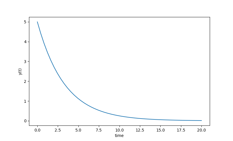
An example of using ODEINT is with the following differential equation with parameter k=0.3, the initial condition y0=5 and the following differential equation.
The Python code first imports the needed Numpy, Scipy, and Matplotlib packages. The model, initial conditions, and time points are defined as inputs to ODEINT to numerically calculate y(t).
import numpy as np
from scipy. integrate import odeint
import matplotlib. pyplot as plt
# function that returns dy/dt
def model ( y , t ) :
k = 0.3
dydt = -k * y
return dydt
# time points
t = np. linspace ( 0 , 20 )
# solve ODE
y = odeint ( model , y0 , t )
# plot results
plt. plot ( t , y )
plt. xlabel ( ‘time’ )
plt. ylabel ( ‘y(t)’ )
plt. show ( )
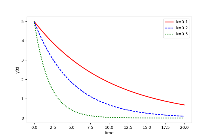
An optional fourth input is args that allows additional information to be passed into the model function. The args input is a tuple sequence of values. The argument k is now an input to the model function by including an addition argument.
import numpy as np
from scipy. integrate import odeint
import matplotlib. pyplot as plt
# function that returns dy/dt
def model ( y , t , k ) :
dydt = -k * y
return dydt
# time points
t = np. linspace ( 0 , 20 )
# solve ODEs
k = 0.1
y1 = odeint ( model , y0 , t , args = ( k , ) )
k = 0.2
y2 = odeint ( model , y0 , t , args = ( k , ) )
k = 0.5
y3 = odeint ( model , y0 , t , args = ( k , ) )
# plot results
plt. plot ( t , y1 , ‘r-‘ , linewidth = 2 , label = ‘k=0.1’ )
plt. plot ( t , y2 , ‘b—‘ , linewidth = 2 , label = ‘k=0.2’ )
plt. plot ( t , y3 , ‘g:’ , linewidth = 2 , label = ‘k=0.5’ )
plt. xlabel ( ‘time’ )
plt. ylabel ( ‘y(t)’ )
plt. legend ( )
plt. show ( )
Exercises
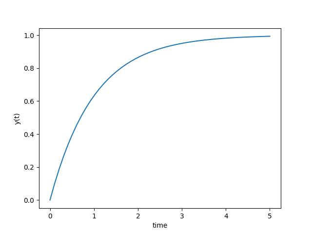
Find a numerical solution to the following differential equations with the associated initial conditions. Expand the requested time horizon until the solution reaches a steady state. Show a plot of the states (x(t) and/or y(t)). Report the final value of each state as `t \to \infty`.
import numpy as np
from scipy. integrate import odeint
import matplotlib. pyplot as plt
# function that returns dy/dt
def model ( y , t ) :
dydt = -y + 1.0
return dydt
# time points
t = np. linspace ( 0 , 5 )
# solve ODE
y = odeint ( model , y0 , t )
# plot results
plt. plot ( t , y )
plt. xlabel ( ‘time’ )
plt. ylabel ( ‘y(t)’ )
plt. show ( )
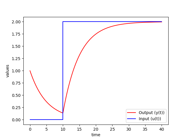
`u` steps from 0 to 2 at `t=10`
import numpy as np
from scipy. integrate import odeint
import matplotlib. pyplot as plt
# function that returns dy/dt
def model ( y , t ) :
# u steps from 0 to 2 at t=10
if t < 10.0 :
u = 0
else :
u = 2
dydt = ( -y + u ) / 5.0
return dydt
# time points
t = np. linspace ( 0 , 40 , 1000 )
# solve ODE
y = odeint ( model , y0 , t )
# plot results
plt. plot ( t , y , ‘r-‘ , label = ‘Output (y(t))’ )
plt. plot ( [ 0 , 10 , 10 , 40 ] , [ 0 , 0 , 2 , 2 ] , ‘b-‘ , label = ‘Input (u(t))’ )
plt. ylabel ( ‘values’ )
plt. xlabel ( ‘time’ )
plt. legend ( loc = ‘best’ )
plt. show ( )
Solve for `x(t)` and `y(t)` and show that the solutions are equivalent.
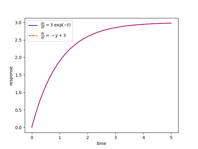
import numpy as np
from scipy. integrate import odeint
import matplotlib. pyplot as plt
# function that returns dz/dt
def model ( z , t ) :
dxdt = 3.0 * np. exp ( -t )
dydt = -z [ 1 ] + 3
dzdt = [ dxdt , dydt ]
return dzdt
# initial condition
z0 = [ 0 , 0 ]
# time points
t = np. linspace ( 0 , 5 )
# solve ODE
z = odeint ( model , z0 , t )
# plot results
plt. plot ( t , z [ : , 0 ] , ‘b-‘ , label = r ‘$ \f rac=3 \; \e xp(-t)$’ )
plt. plot ( t , z [ : , 1 ] , ‘r—‘ , label = r ‘$ \f rac=-y+3$’ )
plt. ylabel ( ‘response’ )
plt. xlabel ( ‘time’ )
plt. legend ( loc = ‘best’ )
plt. show ( )
where `S(t-5)` is a step function that changes from zero to one at `t=5`. When it is multiplied by two, it changes from zero to two at that same time, `t=5`.
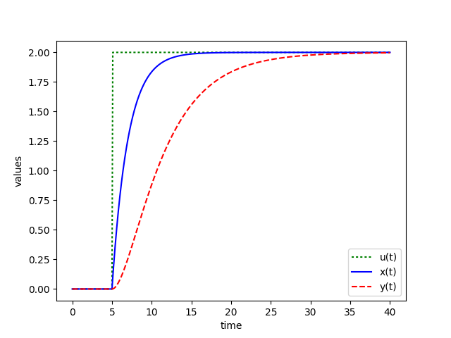
import numpy as np
from scipy. integrate import odeint
import matplotlib. pyplot as plt
# function that returns dz/dt
def model ( z , t , u ) :
x = z [ 0 ]
y = z [ 1 ]
dxdt = ( -x + u ) / 2.0
dydt = ( -y + x ) / 5.0
dzdt = [ dxdt , dydt ]
return dzdt
# initial condition
z0 = [ 0 , 0 ]
# number of time points
n = 401
# time points
t = np. linspace ( 0 , 40 , n )
# step input
u = np. zeros ( n )
# change to 2.0 at time = 5.0
u [ 50 : ] = 2.0
# store solution
x = np. empty_like ( t )
y = np. empty_like ( t )
# record initial conditions
x [ 0 ] = z0 [ 0 ]
y [ 0 ] = z0 [ 1 ]
# solve ODE
for i in range ( 1 , n ) :
# span for next time step
tspan = [ t [ i- 1 ] , t [ i ] ]
# solve for next step
z = odeint ( model , z0 , tspan , args = ( u [ i ] , ) )
# store solution for plotting
x [ i ] = z [ 1 ] [ 0 ]
y [ i ] = z [ 1 ] [ 1 ]
# next initial condition
z0 = z [ 1 ]
# plot results
plt. plot ( t , u , ‘g:’ , label = ‘u(t)’ )
plt. plot ( t , x , ‘b-‘ , label = ‘x(t)’ )
plt. plot ( t , y , ‘r—‘ , label = ‘y(t)’ )
plt. ylabel ( ‘values’ )
plt. xlabel ( ‘time’ )
plt. legend ( loc = ‘best’ )
plt. show ( )