- Python 3: Генерация случайных чисел (модуль random)
- random.random
- random.seed
- random.uniform
- random.randint
- random.choince
- random.randrange
- random.shuffle
- Вероятностные распределения
- Примеры
- Генерация произвольного пароля
- Ссылки
- numpy.random.normal#
- numpy.random.normal#
- Метод numpy.random.normal() — случайные выборки в Python
- Синтаксис
- Аргументы
- Пример 1 numpy.random.normal()
- Пример 2
Python 3: Генерация случайных чисел (модуль random)
Python порождает случайные числа на основе формулы, так что они не на самом деле случайные, а, как говорят, псевдослучайные [1]. Этот способ удобен для большинства приложений (кроме онлайновых казино) [2].
| [1] | Википедия: Генератор псевдослучайных чисел |
| [2] | Доусон М. Программируем на Python. — СПб.: Питер, 2014. — 416 с.: ил. — 3-е изд |
Модуль random позволяет генерировать случайные числа. Прежде чем использовать модуль, необходимо подключить его с помощью инструкции:
random.random
random.random() — возвращает псевдослучайное число от 0.0 до 1.0
random.random() 0.07500815468466127
random.seed
random.seed() — настраивает генератор случайных чисел на новую последовательность. По умолчанию используется системное время. Если значение параметра будет одиноким, то генерируется одинокое число:
random.seed(20) random.random() 0.9056396761745207 random.random() 0.6862541570267026 random.seed(20) random.random() 0.9056396761745207 random.random() 0.7665092563626442
random.uniform
random.uniform(, ) — возвращает псевдослучайное вещественное число в диапазоне от до :
random.uniform(0, 20) 15.330185127252884 random.uniform(0, 20) 18.092324756265473
random.randint
random.randint(, ) — возвращает псевдослучайное целое число в диапазоне от до :
random.randint(1,27) 9 random.randint(1,27) 22
random.choince
random.choince() — возвращает случайный элемент из любой последовательности (строки, списка, кортежа):
random.choice('Chewbacca') 'h' random.choice([1,2,'a','b']) 2 random.choice([1,2,'a','b']) 'a'
random.randrange
random.randrange(, , ) — возвращает случайно выбранное число из последовательности.
random.shuffle
random.shuffle() — перемешивает последовательность (изменяется сама последовательность). Поэтому функция не работает для неизменяемых объектов.
List = [1,2,3,4,5,6,7,8,9] List [1, 2, 3, 4, 5, 6, 7, 8, 9] random.shuffle(List) List [6, 7, 1, 9, 5, 8, 3, 2, 4]
Вероятностные распределения
random.triangular(low, high, mode) — случайное число с плавающей точкой, low ≤ N ≤ high . Mode — распределение.
random.betavariate(alpha, beta) — бета-распределение. alpha>0 , beta>0 . Возвращает от 0 до 1.
random.expovariate(lambd) — экспоненциальное распределение. lambd равен 1/среднее желаемое. Lambd должен быть отличным от нуля. Возвращаемые значения от 0 до плюс бесконечности, если lambd положительно, и от минус бесконечности до 0, если lambd отрицательный.
random.gammavariate(alpha, beta) — гамма-распределение. Условия на параметры alpha>0 и beta>0 .
random.gauss(значение, стандартное отклонение) — распределение Гаусса.
random.lognormvariate(mu, sigma) — логарифм нормального распределения. Если взять натуральный логарифм этого распределения, то вы получите нормальное распределение со средним mu и стандартным отклонением sigma . mu может иметь любое значение, и sigma должна быть больше нуля.
random.normalvariate(mu, sigma) — нормальное распределение. mu — среднее значение, sigma — стандартное отклонение.
random.vonmisesvariate(mu, kappa) — mu — средний угол, выраженный в радианах от 0 до 2π, и kappa — параметр концентрации, который должен быть больше или равен нулю. Если каппа равна нулю, это распределение сводится к случайному углу в диапазоне от 0 до 2π.
random.paretovariate(alpha) — распределение Парето.
random.weibullvariate(alpha, beta) — распределение Вейбулла.
Примеры
Генерация произвольного пароля
Хороший пароль должен быть произвольным и состоять минимум из 6 символов, в нём должны быть цифры, строчные и прописные буквы. Приготовить такой пароль можно по следующему рецепту:
import random # Щепотка цифр str1 = '123456789' # Щепотка строчных букв str2 = 'qwertyuiopasdfghjklzxcvbnm' # Щепотка прописных букв. Готовится преобразованием str2 в верхний регистр. str3 = str2.upper() print(str3) # Выведет: 'QWERTYUIOPASDFGHJKLZXCVBNM' # Соединяем все строки в одну str4 = str1+str2+str3 print(str4) # Выведет: '123456789qwertyuiopasdfghjklzxcvbnmQWERTYUIOPASDFGHJKLZXCVBNM' # Преобразуем получившуюся строку в список ls = list(str4) # Тщательно перемешиваем список random.shuffle(ls) # Извлекаем из списка 12 произвольных значений psw = ''.join([random.choice(ls) for x in range(12)]) # Пароль готов print(psw) # Выведет: '1t9G4YPsQ5L7'
Этот же скрипт можно записать всего в две строки:
import random print(''.join([random.choice(list('123456789qwertyuiopasdfghjklzxc vbnmQWERTYUIOPASDFGHJKLZXCVBNM')) for x in range(12)]))
Данная команда является краткой записью цикла for, вместо неё можно было написать так:
import random psw = '' # предварительно создаем переменную psw for x in range(12): psw = psw + random.choice(list('123456789qwertyuiopasdfgh jklzxcvbnmQWERTYUIOPASDFGHJKLZXCVBNM')) print(psw) # Выведет: Ci7nU6343YGZ
Данный цикл повторяется 12 раз и на каждом круге добавляет к строке psw произвольно выбранный элемент из списка.
Ссылки
numpy.random.normal#
Draw random samples from a normal (Gaussian) distribution.
The probability density function of the normal distribution, first derived by De Moivre and 200 years later by both Gauss and Laplace independently [2], is often called the bell curve because of its characteristic shape (see the example below).
The normal distributions occurs often in nature. For example, it describes the commonly occurring distribution of samples influenced by a large number of tiny, random disturbances, each with its own unique distribution [2].
New code should use the normal method of a Generator instance instead; please see the Quick Start .
Mean (“centre”) of the distribution.
scale float or array_like of floats
Standard deviation (spread or “width”) of the distribution. Must be non-negative.
size int or tuple of ints, optional
Output shape. If the given shape is, e.g., (m, n, k) , then m * n * k samples are drawn. If size is None (default), a single value is returned if loc and scale are both scalars. Otherwise, np.broadcast(loc, scale).size samples are drawn.
Returns : out ndarray or scalar
Drawn samples from the parameterized normal distribution.
probability density function, distribution or cumulative density function, etc.
which should be used for new code.
The probability density for the Gaussian distribution is
where \(\mu\) is the mean and \(\sigma\) the standard deviation. The square of the standard deviation, \(\sigma^2\) , is called the variance.
The function has its peak at the mean, and its “spread” increases with the standard deviation (the function reaches 0.607 times its maximum at \(x + \sigma\) and \(x — \sigma\) [2]). This implies that normal is more likely to return samples lying close to the mean, rather than those far away.
P. R. Peebles Jr., “Central Limit Theorem” in “Probability, Random Variables and Random Signal Principles”, 4th ed., 2001, pp. 51, 51, 125.
Draw samples from the distribution:
>>> mu, sigma = 0, 0.1 # mean and standard deviation >>> s = np.random.normal(mu, sigma, 1000)
Verify the mean and the variance:
>>> abs(mu - np.mean(s)) 0.0 # may vary
>>> abs(sigma - np.std(s, ddof=1)) 0.1 # may vary
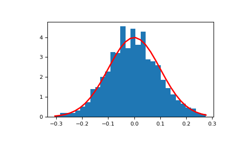
Display the histogram of the samples, along with the probability density function:
>>> import matplotlib.pyplot as plt >>> count, bins, ignored = plt.hist(s, 30, density=True) >>> plt.plot(bins, 1/(sigma * np.sqrt(2 * np.pi)) * . np.exp( - (bins - mu)**2 / (2 * sigma**2) ), . linewidth=2, color='r') >>> plt.show()
Two-by-four array of samples from the normal distribution with mean 3 and standard deviation 2.5:
>>> np.random.normal(3, 2.5, size=(2, 4)) array([[-4.49401501, 4.00950034, -1.81814867, 7.29718677], # random [ 0.39924804, 4.68456316, 4.99394529, 4.84057254]]) # random
numpy.random.normal#
Draw random samples from a normal (Gaussian) distribution.
The probability density function of the normal distribution, first derived by De Moivre and 200 years later by both Gauss and Laplace independently [2], is often called the bell curve because of its characteristic shape (see the example below).
The normal distributions occurs often in nature. For example, it describes the commonly occurring distribution of samples influenced by a large number of tiny, random disturbances, each with its own unique distribution [2].
New code should use the normal method of a Generator instance instead; please see the Quick Start .
Mean (“centre”) of the distribution.
scale float or array_like of floats
Standard deviation (spread or “width”) of the distribution. Must be non-negative.
size int or tuple of ints, optional
Output shape. If the given shape is, e.g., (m, n, k) , then m * n * k samples are drawn. If size is None (default), a single value is returned if loc and scale are both scalars. Otherwise, np.broadcast(loc, scale).size samples are drawn.
Returns : out ndarray or scalar
Drawn samples from the parameterized normal distribution.
probability density function, distribution or cumulative density function, etc.
which should be used for new code.
The probability density for the Gaussian distribution is
where \(\mu\) is the mean and \(\sigma\) the standard deviation. The square of the standard deviation, \(\sigma^2\) , is called the variance.
The function has its peak at the mean, and its “spread” increases with the standard deviation (the function reaches 0.607 times its maximum at \(x + \sigma\) and \(x — \sigma\) [2]). This implies that normal is more likely to return samples lying close to the mean, rather than those far away.
P. R. Peebles Jr., “Central Limit Theorem” in “Probability, Random Variables and Random Signal Principles”, 4th ed., 2001, pp. 51, 51, 125.
Draw samples from the distribution:
>>> mu, sigma = 0, 0.1 # mean and standard deviation >>> s = np.random.normal(mu, sigma, 1000)
Verify the mean and the variance:
>>> abs(mu - np.mean(s)) 0.0 # may vary
>>> abs(sigma - np.std(s, ddof=1)) 0.1 # may vary
Display the histogram of the samples, along with the probability density function:
>>> import matplotlib.pyplot as plt >>> count, bins, ignored = plt.hist(s, 30, density=True) >>> plt.plot(bins, 1/(sigma * np.sqrt(2 * np.pi)) * . np.exp( - (bins - mu)**2 / (2 * sigma**2) ), . linewidth=2, color='r') >>> plt.show()

Two-by-four array of samples from the normal distribution with mean 3 and standard deviation 2.5:
>>> np.random.normal(3, 2.5, size=(2, 4)) array([[-4.49401501, 4.00950034, -1.81814867, 7.29718677], # random [ 0.39924804, 4.68456316, 4.99394529, 4.84057254]]) # random
Метод numpy.random.normal() — случайные выборки в Python
Функция numpy.random.normal() выполняет случайные выборки и генерирует случайные значения из нормального (гауссовского) распределения в Python.
Нормальное распределение часто называют кривой нормального распределения из-за его формы. Поскольку форма графика нормального распределения похожа на колокол, его часто называют кривой колокола.
Синтаксис
Аргументы
- loc: Это среднее значение нормального распределения. Его также называют средним. Если в аргументе ничего не передается, он автоматически принимает 0 в качестве среднего значения для нормального распределения. Потому что если получается нормальное распределение, то среднее значение равно 0; поэтому 0.0 назначается по умолчанию.
- scale: Это стандартное отклонение нормального распределения. Его также называют стандартным отклонением. Как следует из названия, это стандартное отклонение между точками нормального распределения. Если в качестве аргумента передается стандартное отклонение, функция автоматически присваивает значение 1,0.
- size: это количество отрисовываемых образцов. Если n — количество выборок, переданных в аргументе, то выбирается n выборок. Если в аргументе ничего не указано, будет взята 1 выборка.
Пример 1 numpy.random.normal()
В этой программе мы импортировали пакет numpy, состоящий из нескольких функций. Мы использовали функцию random.normal(). Это функция, присутствующая внутри случайного класса пакета numpy. Функция np.random.normal() находит нормальное распределение для случайных выборок.
Пример 2
В этой программе мы создали три переменные: mu, sigma и siz.
mu используется для хранения среднего значения нормального распределения. Sigma используется для хранения стандартного отклонения. А siz используется для хранения количества выборок.
Мы передали функции среднее значение, стандартное отклонение и размер. Следовательно, на выходе будет семь выборок, поскольку мы указали семь в качестве размера.

Автор статей и разработчик, делюсь знаниями.