Import the numpy library and define a custom dataset x and y of equal length:
Python3 Define the correlation by applying the above formula: Python3 The above output shows that the relationship between x and y is 0.974894414261588 and x and x is 1.0
We can also find the correlation by using the numpy corrcoef function.
Python3 The above output shows the correlations between x&x, x&y, y&x, and y&y.
Example Import the necessary libraries Python3 Loading load_diabetes Data from sklearn.dataset Python3 age sex bmi bp s1 s2 s3 s4 s5 s6 target 0 0.038076 0.050680 0.061696 0.021872 -0.044223 -0.034821 -0.043401 -0.002592 0.019907 -0.017646 1 -0.001882 -0.044642 -0.051474 -0.026328 -0.008449 -0.019163 0.074412 -0.039493 -0.068332 -0.092204 2 0.085299 0.050680 0.044451 -0.005670 -0.045599 -0.034194 -0.032356 -0.002592 0.002861 -0.025930 3 -0.089063 -0.044642 -0.011595 -0.036656 0.012191 0.024991 -0.036038 0.034309 0.022688 -0.009362 4 0.005383 -0.044642 -0.036385 0.021872 0.003935 0.015596 0.008142 -0.002592 -0.031988 -0.046641
Find the Pearson correlations matrix by using the pandas command df.corr() df.corr(method, min_periods,numeric_only ) method : In method we can choose any one from pearson is the standard correlation coefficient matrix i.e default min_periods : int This is optional. Defines th eminimum number of observations required per pair. numeric_only : Default is False, Defines we want to compare only numeric or categorical object also Python3 age sex bmi bp s1 s2 s3 s4 s5 s6 target age 1.000000 0.173737 0.185085 0.335428 0.260061 0.219243 -0.075181 0.203841 0.270774 0.301731 0.187889 sex 0.173737 1.000000 0.088161 0.241010 0.035277 0.142637 -0.379090 0.332115 0.149916 0.208133 0.043062 bmi 0.185085 0.088161 1.000000 0.395411 0.249777 0.261170 -0.366811 0.413807 0.446157 0.388680 0.586450 bp 0.335428 0.241010 0.395411 1.000000 0.242464 0.185548 -0.178762 0.257650 0.393480 0.390430 0.441482 s1 0.260061 0.035277 0.249777 0.242464 1.000000 0.896663 0.051519 0.542207 0.515503 0.325717 0.212022 s2 0.219243 0.142637 0.261170 0.185548 0.896663 1.000000 -0.196455 0.659817 0.318357 0.290600 0.174054 s3 -0.075181 -0.379090 -0.366811 -0.178762 0.051519 -0.196455 1.000000 -0.738493 -0.398577 -0.273697 -0.394789 s4 0.203841 0.332115 0.413807 0.257650 0.542207 0.659817 -0.738493 1.000000 0.617859 0.417212 0.430453 s5 0.270774 0.149916 0.446157 0.393480 0.515503 0.318357 -0.398577 0.617859 1.000000 0.464669 0.565883 s6 0.301731 0.208133 0.388680 0.390430 0.325717 0.290600 -0.273697 0.417212 0.464669 1.000000 0.382483 target 0.187889 0.043062 0.586450 0.441482 0.212022 0.174054 -0.394789 0.430453 0.565883 0.382483 1.000000
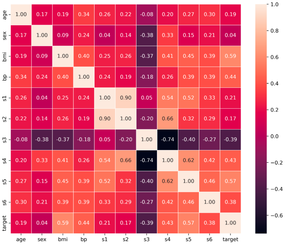
The above table represents the correlations between each column of the data frame. The correlation between the self is 1.0, The negative correlation defined negative relationship means on increasing one column value second will decrease and vice-versa. The zeros correlation defines no relationship I.e neutral. and positive correlations define positive relationships meaning on increasing one column value second will also increase and vice-versa.
We can also find the correlations using numpy between two columns
Python3 Correlations between Age and Sex [[1. 0.1737371] [0.1737371 1. ]] We can match from the above correlation matrix table, it is almost the same result.
Plot the correlation matrix with the seaborn heatmap Python3
Improve your Coding Skills with Practice
Computer Science GATE CS Notes Operating Systems Computer Network Database Management System Software Engineering Digital Logic Design Engineering Maths Python Python Programming Examples Django Tutorial Python Projects Python Tkinter OpenCV Python Tutorial Python Interview Question Data Science & ML Data Science With Python Data Science For Beginner Machine Learning Tutorial Maths For Machine Learning Pandas Tutorial NumPy Tutorial NLP Tutorial Deep Learning Tutorial DevOps Git AWS Docker Kubernetes Azure GCP Competitive Programming Top DSA for CP Top 50 Tree Problems Top 50 Graph Problems Top 50 Array Problems Top 50 String Problems Top 50 DP Problems Top 15 Websites for CP System Design What is System Design Monolithic and Distributed SD Scalability in SD Databases in SD High Level Design or HLD Low Level Design or LLD Top SD Interview Questions Interview Corner Company Wise Preparation Preparation for SDE Experienced Interviews Internship Interviews Competitive Programming Aptitude Preparation GfG School CBSE Notes for Class 8 CBSE Notes for Class 9 CBSE Notes for Class 10 CBSE Notes for Class 11 CBSE Notes for Class 12 English Grammar Commerce Accountancy Business Studies Economics Management Income Tax Finance UPSC Polity Notes Geography Notes History Notes Science and Technology Notes Economics Notes Important Topics in Ethics UPSC Previous Year Papers SSC/ BANKING SSC CGL Syllabus SBI PO Syllabus SBI Clerk Syllabus IBPS PO Syllabus IBPS Clerk Syllabus Aptitude Questions SSC CGL Practice Papers Write & Earn Write an Article Improve an Article Pick Topics to Write Write Interview Experience Internships Video Internship We use cookies to ensure you have the best browsing experience on our website. By using our site, you acknowledge that you have read and understood our Cookie Policy & Privacy Policy Got It !
This article is being improved by another user right now. You can suggest the changes for now and it will be under the article’s discussion tab.
You will be notified via email once the article is available for improvement. Thank you for your valuable feedback!
Help us improve. Share your suggestions to enhance the article. Contribute your expertise and make a difference in the GeeksforGeeks portal.
Enhance the article with your expertise. Contribute to the GeeksforGeeks community and help create better learning resources for all.
Источник
numpy.corrcoef# Return Pearson product-moment correlation coefficients.
Please refer to the documentation for cov for more detail. The relationship between the correlation coefficient matrix, R , and the covariance matrix, C , is
The values of R are between -1 and 1, inclusive.
Parameters : x array_like
A 1-D or 2-D array containing multiple variables and observations. Each row of x represents a variable, and each column a single observation of all those variables. Also see rowvar below.
y array_like, optional
An additional set of variables and observations. y has the same shape as x .
rowvar bool, optional
If rowvar is True (default), then each row represents a variable, with observations in the columns. Otherwise, the relationship is transposed: each column represents a variable, while the rows contain observations.
bias _NoValue, optional
Deprecated since version 1.10.0.
Deprecated since version 1.10.0.
Data-type of the result. By default, the return data-type will have at least numpy.float64 precision.
The correlation coefficient matrix of the variables.
Due to floating point rounding the resulting array may not be Hermitian, the diagonal elements may not be 1, and the elements may not satisfy the inequality abs(a)
This function accepts but discards arguments bias and ddof . This is for backwards compatibility with previous versions of this function. These arguments had no effect on the return values of the function and can be safely ignored in this and previous versions of numpy.
In this example we generate two random arrays, xarr and yarr , and compute the row-wise and column-wise Pearson correlation coefficients, R . Since rowvar is true by default, we first find the row-wise Pearson correlation coefficients between the variables of xarr .
>>> import numpy as np >>> rng = np . random . default_rng ( seed = 42 ) >>> xarr = rng . random (( 3 , 3 )) >>> xarr array([[0.77395605, 0.43887844, 0.85859792], [0.69736803, 0.09417735, 0.97562235], [0.7611397 , 0.78606431, 0.12811363]]) >>> R1 = np . corrcoef ( xarr ) >>> R1 array([[ 1. , 0.99256089, -0.68080986], [ 0.99256089, 1. , -0.76492172], [-0.68080986, -0.76492172, 1. ]]) If we add another set of variables and observations yarr , we can compute the row-wise Pearson correlation coefficients between the variables in xarr and yarr .
>>> yarr = rng . random (( 3 , 3 )) >>> yarr array([[0.45038594, 0.37079802, 0.92676499], [0.64386512, 0.82276161, 0.4434142 ], [0.22723872, 0.55458479, 0.06381726]]) >>> R2 = np . corrcoef ( xarr , yarr ) >>> R2 array([[ 1. , 0.99256089, -0.68080986, 0.75008178, -0.934284 , -0.99004057], [ 0.99256089, 1. , -0.76492172, 0.82502011, -0.97074098, -0.99981569], [-0.68080986, -0.76492172, 1. , -0.99507202, 0.89721355, 0.77714685], [ 0.75008178, 0.82502011, -0.99507202, 1. , -0.93657855, -0.83571711], [-0.934284 , -0.97074098, 0.89721355, -0.93657855, 1. , 0.97517215], [-0.99004057, -0.99981569, 0.77714685, -0.83571711, 0.97517215, 1. ]]) Finally if we use the option rowvar=False , the columns are now being treated as the variables and we will find the column-wise Pearson correlation coefficients between variables in xarr and yarr .
>>> R3 = np . corrcoef ( xarr , yarr , rowvar = False ) >>> R3 array([[ 1. , 0.77598074, -0.47458546, -0.75078643, -0.9665554 , 0.22423734], [ 0.77598074, 1. , -0.92346708, -0.99923895, -0.58826587, -0.44069024], [-0.47458546, -0.92346708, 1. , 0.93773029, 0.23297648, 0.75137473], [-0.75078643, -0.99923895, 0.93773029, 1. , 0.55627469, 0.47536961], [-0.9665554 , -0.58826587, 0.23297648, 0.55627469, 1. , -0.46666491], [ 0.22423734, -0.44069024, 0.75137473, 0.47536961, -0.46666491, 1. ]]) Источник