Python normal distribution pdf

scipy.stats.norm#

The location ( loc ) keyword specifies the mean. The scale ( scale ) keyword specifies the standard deviation.

As an instance of the rv_continuous class, norm object inherits from it a collection of generic methods (see below for the full list), and completes them with details specific for this particular distribution.

The probability density function for norm is:

The probability density above is defined in the “standardized” form. To shift and/or scale the distribution use the loc and scale parameters. Specifically, norm.pdf(x, loc, scale) is identically equivalent to norm.pdf(y) / scale with y = (x — loc) / scale . Note that shifting the location of a distribution does not make it a “noncentral” distribution; noncentral generalizations of some distributions are available in separate classes.

>>> import numpy as np >>> from scipy.stats import norm >>> import matplotlib.pyplot as plt >>> fig, ax = plt.subplots(1, 1) 

Calculate the first four moments:

>>> mean, var, skew, kurt = norm.stats(moments='mvsk') 

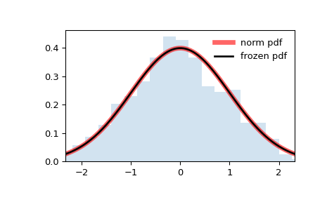
Display the probability density function ( pdf ):

>>> x = np.linspace(norm.ppf(0.01), . norm.ppf(0.99), 100) >>> ax.plot(x, norm.pdf(x), . 'r-', lw=5, alpha=0.6, label='norm pdf') 

Alternatively, the distribution object can be called (as a function) to fix the shape, location and scale parameters. This returns a “frozen” RV object holding the given parameters fixed.

Freeze the distribution and display the frozen pdf :

>>> rv = norm() >>> ax.plot(x, rv.pdf(x), 'k-', lw=2, label='frozen pdf') 

Check accuracy of cdf and ppf :

>>> vals = norm.ppf([0.001, 0.5, 0.999]) >>> np.allclose([0.001, 0.5, 0.999], norm.cdf(vals)) True 

And compare the histogram:

>>> ax.hist(r, density=True, bins='auto', histtype='stepfilled', alpha=0.2) >>> ax.set_xlim([x[0], x[-1]]) >>> ax.legend(loc='best', frameon=False) >>> plt.show() 

rvs(loc=0, scale=1, size=1, random_state=None)

pdf(x, loc=0, scale=1)

Probability density function.

logpdf(x, loc=0, scale=1)

Log of the probability density function.

cdf(x, loc=0, scale=1)

Cumulative distribution function.

logcdf(x, loc=0, scale=1)

Log of the cumulative distribution function.

sf(x, loc=0, scale=1)

Survival function (also defined as 1 — cdf , but sf is sometimes more accurate).

logsf(x, loc=0, scale=1)

Log of the survival function.

ppf(q, loc=0, scale=1)

Percent point function (inverse of cdf — percentiles).

isf(q, loc=0, scale=1)

Inverse survival function (inverse of sf ).

moment(order, loc=0, scale=1)

Non-central moment of the specified order.

stats(loc=0, scale=1, moments=’mv’)

Mean(‘m’), variance(‘v’), skew(‘s’), and/or kurtosis(‘k’).

entropy(loc=0, scale=1)

(Differential) entropy of the RV.

Parameter estimates for generic data. See scipy.stats.rv_continuous.fit for detailed documentation of the keyword arguments.

expect(func, args=(), loc=0, scale=1, lb=None, ub=None, conditional=False, **kwds)

Expected value of a function (of one argument) with respect to the distribution.

median(loc=0, scale=1)

Median of the distribution.

mean(loc=0, scale=1)

var(loc=0, scale=1)

Variance of the distribution.

std(loc=0, scale=1)

Standard deviation of the distribution.

interval(confidence, loc=0, scale=1)

Confidence interval with equal areas around the median.

Источник

Normal Distribution: A Practical Guide Using Python and SciPy

We recently discussed the basics of Normal Distribution and its distinctive features. It’s time to apply that theory and gain hands-on experience.

In this post, you’ll learn how to:

• Create normal distribution using Python and SciPy.
• Generate samples of a normally distributed variable.
• Calculate percentiles and find probabilities for specific values.
• Plot histogram, density curve, and area under the curve.

Normal Distribution Using SciPy 🔗

SciPy’s stats module provides a large number of statistics functions. The class norm from this module implements normal distribution.

Let’s explore this class using an example.

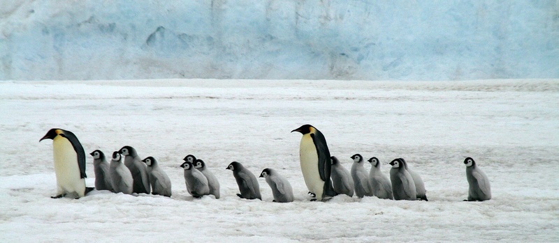
Photo Credit: bdougherty

Emperor penguins are the tallest among all the penguin species. Suppose their height is normally distributed with a mean of 40 inches and a standard deviation of 5 inches.

Let’s use the class norm to create the height distribution. The class takes mean and standard deviation as the inputs:

# load scipy's statistics module from scipy import stats # Emperor penguins height statistics (in inches) mean = 40 standard_deviation = 5 # Create normal distribution using the 'norm' class # loc - specifies the mean # scale - specifies the standard deviation height_distribution = stats.norm( loc=mean, scale=standard_deviation ) 

You can use the returned object ( height_distribution ) to perform various operations related to normal distribution. We’ll look at some of the most popular ones.

Random Sample Using rvs() 🔗

Suppose you want a sample of 20 height measurements selected at random. You can do that using norm’s rvs() method:

# Generate a sample of 20 random penguin heights sample = height_distribution.rvs(size=20) sample.round(2) 

array([36.82, 42.66, 44.95, 36.88, 47.34, 42.03, 46.49, 26.93, 46.78, 49.37, 39.51, 42.82, 40.85, 43.91, 44.33, 39.7 , 36.57, 40.86, 33.53, 42.64]) 

The sample heights seem reasonable. But is rvs() creating normally distributed values? To confirm, let’s generate a larger sample of 3,000 measurements and plot a histogram:

### Generate 3000 heights measurements # height_distribution is an instance of 'norm' class # Use its method rvs() to get the sample sample = height_distribution.rvs(size=3000) 

### Plot sample heights as histogram # import matplotlib and seaborn for visualization import matplotlib.pyplot as plt import seaborn as sns # Use seaborn style and increase font size sns.set_theme(style='ticks', font_scale=1.5) # set figure dimensions plt.figure(figsize=(12, 6)) # Plot histogram # Use larger bin count (100) to get smoother shape plt.hist(sample, bins=100) plt.title("Emperor Penguin Heights - Histogram", pad=20) plt.xlabel("Height (inches)", labelpad=10) plt.ylabel("Frequency", labelpad=10) plt.show()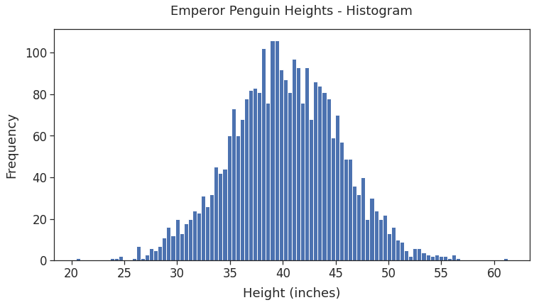 

The generated values are indeed normally distributed! The heights of most penguins are clustered around the mean (40 inches). And the frequency decreases as the height gets farther from the mean in either direction.

Probability of a Given Value Using pdf() 🔗

Let’s say you want to find out:

What’s the probability that a randomly selected penguin will be 40 inches tall?

The method pdf() from the norm class can help us answer such questions. It returns the probabilities for specific values from a normal distribution. (PDF stands for Probability Density Function)

Here’s how you can use pdf():

# Find probability that a penguin is 40 inches tall probability_40 = height_distribution.pdf(x=40) probability_40.round(4) 

Thus, there’s a 7.98% chance that a randomly selected penguin is 40 inches tall.

Density Curve Using pdf() 🔗

A density curve is a graphical plot showing probabilities associated with different values of a variable. Let’s use pdf() to plot the density curve for the penguin heights.

First, we’ll pick 1,000 height measurements between 20 and 60 inches. We can do that using NumPy’s linspace():

# load numpy import numpy as np # Get 1000 evenly spaced heights between # 20 and 60 inches using numpy's linspace() min_height = 20 max_height = 60 height_values = np.linspace(min_height, max_height, num=1000) # print size, first 10 and last 10 values print("Height Values Count: ", height_values.size) print("Head: ", height_values[:10].round(2)) print("Tail: ", height_values[-10:].round(2)) 

Height Values Count: 1000 Head: [20. 20.04 20.08 20.12 20.16 20.2 20.24 20.28 20.32 20.36] Tail: [59.64 59.68 59.72 59.76 59.8 59.84 59.88 59.92 59.96 60. ] 

Next, get the probabilities for all the values using pdf():

# Calculate probabilites using scipy.stats.norm.pdf() probabilities = height_distribution.pdf(x=height_values) 

Finally, plot the heights on the x-axis and the corresponding probabilities on the y-axis. That’ll give you the density curve:

# set graph size plt.figure(figsize=(12, 6)) # plot density curve # heights on x-axis and their probabilities on y-axis plt.plot(height_values, probabilities) # shade the area under the density curve plt.fill_between(height_values, probabilities, alpha=0.2) # Remove the dead space (both vertical and horizontal) # that Matplotlib adds by default axes = plt.gca() axes.set_xlim([min_height, max_height]) ymin, ymax = axes.get_ylim() axes.set_ylim([0, ymax]) # Add figure title, labels plt.title("Emperor Penguin Heights - Density Curve", pad=20) plt.xlabel("Height (inches)", labelpad=10) plt.ylabel("Probability", labelpad=10) plt.show()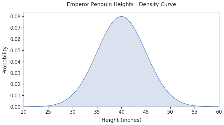 

As expected, we get a smooth density curve that follows the normal distribution.

Find Percent Below a Value Using cdf() 🔗

What percentage of emperor penguins are shorter than 44 inches?

To answer this, you’ll need to add the probabilities of all the heights shorter than 44 inches.

The norm method cdf() can help you do that. The method calculates the proportion of a normally distributed population that is less than or equal to a given value. (CDF stands for Cumulative Distribution Function).

Here’s how you can use cdf():

# How many penguins are shorter than 44 inches? below_44 = height_distribution.cdf(44) below_44.round(4) 

Thus, 78.81% of all emperor penguins are shorter than 44 inches.

Visualize Percent Below a Value 🔗

As we saw above, the x-axis of the density plot has the heights sorted in increasing order. Let’s highlight the region where the height is shorter than 44 inches.

We can do that using Matplotlib’s fill_between() function:

# set graph size plt.figure(figsize=(12, 6)) # plot density curve plt.plot(height_values, probabilities) # Shade the region where height shaded_region = (height_values  44) plt.fill_between(height_values, probabilities, where=shaded_region) # Remove the dead space axes = plt.gca() axes.set_xlim([min_height, max_height]) ymin, ymax = axes.get_ylim() axes.set_ylim([0, ymax]) plt.title("Emperor Penguin Heights - Under 44 Inches", pad=20) plt.xlabel("Height (inches)", labelpad=10) plt.ylabel("Probability", labelpad=10) plt.show()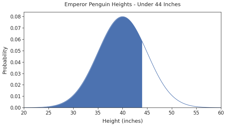 

The shaded region represents the sum of probabilities of heights less than or equal to 44 inches. We found this sum using the cdf() function in the last section. Thus, the shaded region covers 78.81% of the total area under the density curve.

Calculate Percentile Using ppf() 🔗

Let’s say you want to find the height that’ll make a penguin taller than 90% of all emperor penguins. Such a value would be the 90 th percentile for their height distribution.

In general, the N th percentile is the value that is greater than the N percent of all data points.

You can find the percentile using the norm ppf() method. (PPF stands for Percent Point Function). Below code shows how to use ppf():

# scipy.stats.norm.ppf() expects fraction as the input # so pass 0.9 to find 90th percentile percentile_90th = height_distribution.ppf(0.9) percentile_90th.round(2) 

Thus, 46.41 inches is the 90 th percentile height for emperor penguins.

Summary 🔗

This post helped you gain invaluable practical skills using Python and SciPy. Let’s do a quick recap of what you’ve learned:

• Create normal distributions using the norm class from the SciPy stats module.
• Generate random samples using the norm method rvs().
• Calculate probabilities using pdf() and cdf().
• Find percentiles using ppf().
• Plot histogram and density curve for normal distributions using Matplotlib and Seaborn.

Источник