Python create normal distribution

How to Generate a Normal Distribution in Python

The normal distribution is continuous probability distribution for real values random variables whose distributions are not known.

It is one of the important distribution in statistics. Normal distribution is mostly used in social sciences or natural. Normal distribution also known as Gaussian distribution.

A normal distribution is informally called as bell curve.

In this article, we will discuss about how to generate normal distribution in python.

Normal Distribution Definition

A continuous random variable X is said have normal distribution with parameter μ and σ if its probability density function of normal distribution is given by :

We will be using numpy.random.normal() function available to generate normal distribution.

pip install numpy

If you don’t have numpy package installed on your system, installed it using below commands on window system

How to generate a normal distribution

Lets discuss with example to generate normal distribution in python

Lets generate a normal distribution mean = 4 and standard deviation = 2 and sample data of 1000 values

import matplotlib.pyplot as plt import numpy as np #generate sample of 1000 values that follow a normal distribution mean1 = 4 sd1 = 2 data = np.random.normal(mean1,sd1,1000) print(data[0:10]) # Create the bins and histogram count, bins, ignored = plt.hist(data,100,density = True) # Plot the distribution curve plt.plot(bins, 1/(sd1 * np.sqrt(2 * np.pi)) * np.exp( - (bins - mean1)**2 / (2 * sd1 **2)), linewidth =2, color='r') plt.show()

In the above code, first we import numpy package to use normal() function to generate normal distribution.

matplotlib.pyplot package is used to plot histogram to visualize data for generated normal distribution data values.

using data[0:10], it prints first 10 rows of data values.

To visualize distribution data values, we use hist() function to display histogram of the samples data values along with probability density function

[1.54628665 3.72593179 3.38133163 4.20755645 4.02369098 5.07467887 4.247651 3.58789491 2.65753858 6.40072075]

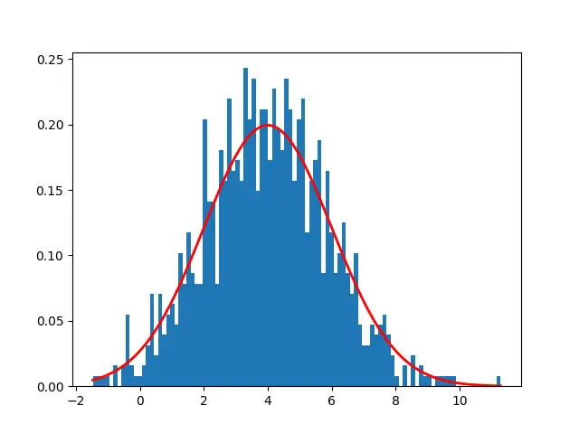
It display first 10 rows of data using data[0:10] and generate histogram plot.

In the above chart, X axis represents random variable, Y axis represent probability of each value, tip of the bell curve is 4 which is mean value.

Example -1 Generate Normal Distribution

Lets generate a normal distribution mean (μ) = 0 and standard deviation (σ) = 1 and sample data of 1000 values

import matplotlib.pyplot as plt import numpy as np #generate sample of 3000 values that follow a normal distribution mean1 = 0 sd1 = 1 data = np.random.normal(mean1,sd1,1000) print(data[0:10]) # Create the bins and histogram count, bins, ignored = plt.hist(data,100,density = True) # Plot the distribution curve plt.plot(bins, 1/(sd1 * np.sqrt(2 * np.pi)) * np.exp( - (bins - mean1)**2 / (2 * sd1 **2)), linewidth =2, color='r') plt.show()

In the above python code to generate normal distribution, we assume mean = 0 and standard deviation = 1, its a specific case and also called as Standard Normal Distribution.

Output of the above python code as below, we have used print(data[0:10]) to print first 10 rows of distribution data.

[ 0.33311452 -0.33228062 0.62564664 -0.64942493 0.91572608 -0.78839538 0.79935677 0.5185406 -0.06801718 -1.61588657]

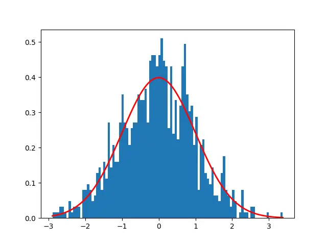
To visualize distribution data values, we have used hist() function which plot chart as below

In the above chart, X axis represents random variable, Y axis represent probability of each value, tip of the bell curve is 0 which is mean value.

Conclusion

I hope you may have liked above article about how to generate normal distribution in python with step by step guide and with illustrative examples.

Recent Posts

Источник

numpy.random.normal#

Draw random samples from a normal (Gaussian) distribution.

The probability density function of the normal distribution, first derived by De Moivre and 200 years later by both Gauss and Laplace independently [2], is often called the bell curve because of its characteristic shape (see the example below).

The normal distributions occurs often in nature. For example, it describes the commonly occurring distribution of samples influenced by a large number of tiny, random disturbances, each with its own unique distribution [2].

New code should use the normal method of a Generator instance instead; please see the Quick Start .

Mean (“centre”) of the distribution.

scale float or array_like of floats

Standard deviation (spread or “width”) of the distribution. Must be non-negative.

size int or tuple of ints, optional

Output shape. If the given shape is, e.g., (m, n, k) , then m * n * k samples are drawn. If size is None (default), a single value is returned if loc and scale are both scalars. Otherwise, np.broadcast(loc, scale).size samples are drawn.

Returns : out ndarray or scalar

Drawn samples from the parameterized normal distribution.

probability density function, distribution or cumulative density function, etc.

which should be used for new code.

The probability density for the Gaussian distribution is

where \(\mu\) is the mean and \(\sigma\) the standard deviation. The square of the standard deviation, \(\sigma^2\) , is called the variance.

The function has its peak at the mean, and its “spread” increases with the standard deviation (the function reaches 0.607 times its maximum at \(x + \sigma\) and \(x — \sigma\) [2]). This implies that normal is more likely to return samples lying close to the mean, rather than those far away.

P. R. Peebles Jr., “Central Limit Theorem” in “Probability, Random Variables and Random Signal Principles”, 4th ed., 2001, pp. 51, 51, 125.

Draw samples from the distribution:

>>> mu, sigma = 0, 0.1 # mean and standard deviation >>> s = np.random.normal(mu, sigma, 1000) 

Verify the mean and the variance:

>>> abs(mu - np.mean(s)) 0.0 # may vary 

>>> abs(sigma - np.std(s, ddof=1)) 0.1 # may vary 

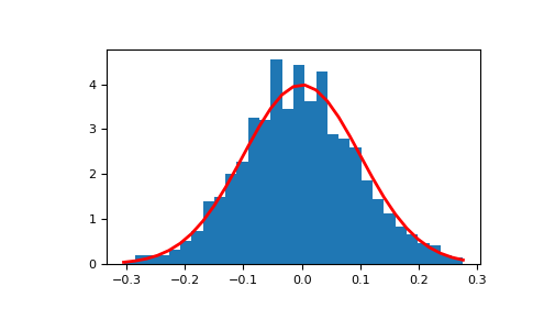
Display the histogram of the samples, along with the probability density function:

>>> import matplotlib.pyplot as plt >>> count, bins, ignored = plt.hist(s, 30, density=True) >>> plt.plot(bins, 1/(sigma * np.sqrt(2 * np.pi)) * . np.exp( - (bins - mu)**2 / (2 * sigma**2) ), . linewidth=2, color='r') >>> plt.show() 

Two-by-four array of samples from the normal distribution with mean 3 and standard deviation 2.5:

>>> np.random.normal(3, 2.5, size=(2, 4)) array([[-4.49401501, 4.00950034, -1.81814867, 7.29718677], # random [ 0.39924804, 4.68456316, 4.99394529, 4.84057254]]) # random 

Источник

Normal Distribution in Python

Even if you’re not a statistician, you’ve probably heard of the term “Normal Distribution” somewhere.

According to probability theory, a random variable’s possible values can be described by its probability distribution. Here, we’re referring to the possible range of values that can be assigned to a parameter based on a random sample.

It is possible to have a probability distribution that is either discrete or constant.

Assume that in a city, the average height of an adult in the 20-30 year old demographic is somewhere between 4.5 and 7 feet tall.

If we were to randomly select one adult and inquire as to his/her height (assuming gender has no bearing on height), what would we discover? It’s impossible to predict the height. Having the height distribution of adults in the city, we can make a more informed bet on what is most likely to happen.

What is Normal Distribution?

A Gaussian distribution, or Bell Curve, is another name for a normal distribution. It’s common practice to use these terms interchangeably, but the meaning is the same in both cases. It is a probability distribution with a wide range of values.

Normal distribution’s probability density function (pdf).

where, σ = Standard deviation, μ = Mean , , x = input value.

• Mean: Ordinary average is referred to as “mean.” Calculated by dividing the sum of all points by the total number of points.
• Standard Deviation: When we look at standard deviation, we can see how “spread out” the information is. Each observed value is compared to the mean to determine how far it deviates from that value.

1. Example Implementation of Normal Distribution

Let’s take a look at the code in the following section. For this demonstration, we’ll make use of NumPy and matplotlib:

# Importing numpy and Matlibplot import numpy as np import matplotlib.pyplot as graph #Creating Data Line till 100 x = np.linspace(1,100,200) #Defining Normal Distribution Function def normalDist(x , mean , sd): prob_density = (np.pi*sd) * np.exp(-0.5*((x-mean)/sd)**2) return prob_density #Mean And Standard deviation Calculation mean = np.mean(x) sd = np.std(x) #Calling Normal Distrubution Function pdf = normalDist(x,mean,sd) #Plotting the Results graph.plot(x,pdf , color = 'blue') graph.xlabel('Discrete Data') graph.ylabel('Probability Density') graph.show()

2. Properties Of Normal Distribution

If we have a data point, along with a mean and standard deviation, the normal distribution density function simply returns a probability density.

We can change the shape of the bell curve by changing the standard deviation and the mean. Changing the mean will cause the curve to move in the direction of the new mean value, allowing us to move the curve’s position while maintaining its original shape.

The Standard deviation has a significant impact on the curve’s appearance. It’s easier to draw a straight line with a smaller standard deviation, but this isn’t always the case.

Properties Of Normal Distribution

• In this case, the mean, median, and mode are all the same.
• The total area under the curve is the same as 1.
• Around the mean, the curve is symmetric.

Empirical rule For Normal Distribution

• The data falls within one standard deviation of the mean in 68% of the cases.
• The majority of the data falls within two standard deviations of the mean equivalent to 95%.
• 99.7% of the data is within three standard deviations of the mean.

It’s one of the most important distributions in all of Statistics. Natural phenomena tend to follow a normal distribution, making the normal distribution magical in that most of them do. Blood pressure, IQ scores, and heights, for example, all fall within the normal distribution.

Using the Normal Distribution to Calculate Probabilities

A normal distribution’s area under the curve can be used to calculate the probability of an individual value occurring in a specific range.

The density function needs to be integrated, so to speak. In a continuous distribution, the area under a normal distribution’s curve represents probabilities. The first thing we need to know about a Standard Normal Distribution is what it is.

To put it another way, the mean and standard deviation of a standard normal distribution are both set to one.

A z-score is another name for the above z value. A z-score tells you how far a data point is from the mean.

To find the cumulative percentage value of our z-value, we must consult a z-table if we intend to perform the probability calculations by hand. Modules in Python take care of all of this for us. Let us now begin.

Create Normal Curve

In order to calculate probabilities based on the normal distribution, we will use the scipy.norm class function.

Consider the following scenario: we have data on the heights of adults in a town that follows a normal distribution; we have a sufficient sample size with a mean of 5.3 and a standard deviation of 1.

Let us see in the below code example the implementation of the Normal Curve.

# Importing scipy, numpy, matplotlib and seaborn from scipy.stats import norm import numpy as np import matplotlib.pyplot as graph import seaborn as sb # Creating the normal Distribution data = np.arange(1,10,0.01) pdf = norm.pdf(data , loc = 5.3 , scale = 1 ) #Plotting the Above Data sb.set_style('whitegrid') sb.lineplot(data, pdf , color = 'red') graph.xlabel('Current Height') graph.ylabel('Probability Density') #Visualizing the Data Plotted Above graph.show()

The probability density value is returned by the norm.pdf() class method, which requires the loc and scale parameters as well as the data as input arguments.

The locator is nothing more than the mean of the data, and the scale is the standard deviation of the data. The code is very similar to what we wrote in the previous section, but it is significantly shorter.

Wrap Up

In this article, we learned about the Normal Distribution, what a normal Curve looks like, and, most importantly, how to implement it in the Python programming environment.

Please let me know if you have any problems or issues with Normal Distribution in the comments section. I would be delighted to assist you as soon as possible.

Источник