Plot pivot table python

Pivot Tables In Python Pandas

For this post, I will be using covid19 database from following link.

Let us first import the necessary packages «requests and pandas».

import requests import pandas as pd import numpy as np 

data = requests.get('https://pomber.github.io/covid19/timeseries.json') 

We need to convert this data to the pandas dataframe so that we can build the pivot table.

columns=['country','date','confirmed','deaths','recovered'] data = [] for country in jsondata: for x in jsondata[country]: data.append([country, x['date'],x['confirmed'],x['deaths'],x['recovered']]) df = pd.DataFrame(data,columns=columns) 

Let us check the number of rows we have in our dataframe by using len(df)

For every country, we have the data of corona virus cases by date.

How to create a pivot table in Python Pandas

Let us create a pivot table with respect to country. Remember we need to pass in the group key that is index for pivot table. Otherwise you would see following error.

ValueError: No group keys passed!

We can sum the numerical data of each country. To do that we can pass np.sum function to the pd.pivot_table().

pivoted = pd.pivot_table(df,index='country',aggfunc=np.sum) 

Let us check the pivot table dataframe now.

Источник

A Guide to Pandas Pivot Table

Pandas’ pivot_table function operates similar to a spreadsheet, making it easier to group, summarize and analyze your data. Here’s how to create your own.

Rebecca Vickery is a data science lead for the energy company EDF, specializing in Python, machine learning, AI and programming. Vickery has worked in data science since 2007. She previously worked as a data scientist for Holiday Extras.

The pandas library is a popular Python package for data analysis. When initially working with a data set in pandas, the structure will be two-dimensional, consisting of rows and columns, which are also known as a DataFrame. An important part of data analysis is the process of grouping, summarizing, aggregating and calculating statistics about this data. Pandas pivot tables provide a powerful tool to perform these analysis techniques with Python.

Create Your Own Pandas Pivot Table in 4 Steps

1. Download or import the data that you want to use.
2. In the pivot_table function, specify the DataFrame you are summarizing, along with the names for the indexes, columns and values.
3. Specify the type of calculation you want to use, such as the mean.
4. Use multiple indexes and column-level grouping to create a more powerful summary of the data.

If you are a spreadsheet user then you may already be familiar with the concept of pivot tables. Pandas pivot tables work in a very similar way to those found in spreadsheet tools such as Microsoft Excel. The pivot table function takes in a data frame and the parameters detailing the shape you want the data to take. Then it outputs summarized data in the form of a pivot table.

I will give a brief introduction with code examples to the pandas pivot table tool. I’ll then use a data set called “autos,” which contains a range of features about cars, such as the make, price, horsepower and miles per gallon.

You can download the data from OpenML, or the code can be imported directly into your code using the scikit-learn API as shown below.

import pandas as pd import numpy as np from sklearn.datasets import fetch_openml X,y = fetch_openml("autos", version=1, as_frame=True, return_X_y=True) data = X data['target'] = y

How to Create a Pandas Pivot Table

A pandas pivot table has three main elements:

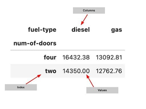
• Index: This specifies the row-level grouping.
• Column: This specifies the column level grouping.
• Values: These are the numerical values you are looking to summarize.

The code used to create the pivot table can be seen below. In the pivot_table function, we specify the DataFrame we are summarizing, and then the column names for the values, index and columns. Additionally, we specify the type of calculation we want to use. In this case, we’re computing the mean.

pivot = np.round(pd.pivot_table(data, values='price', index='num-of-doors', columns='fuel-type', aggfunc=np.mean),2) pivot

Pivot tables can be multi-level. We can use multiple indexes and column level groupings to create more powerful summaries of a data set.

pivot = np.round(pd.pivot_table(data, values='price', index=['num-of-doors', 'body-style'], columns=['fuel-type', 'fuel-system'], aggfunc=np.mean, fill_value=0),2) pivot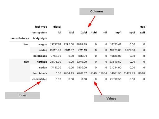

How to Plot with Pandas Pivot Table

Pandas pivot tables can be used in conjunction with the pandas plotting functionality to create useful data visualizations.

Simply adding .plot() to the end of your pivot table code will create a plot of the data. As an example, the below code creates a bar chart showing the mean car price by make and number of doors.

np.round(pd.pivot_table(data, values='price', index=['make'], columns=['num-of-doors'], aggfunc=np.mean, fill_value=0),2).plot.barh(figsize=(10,7), title='Mean car price by make and number of doors')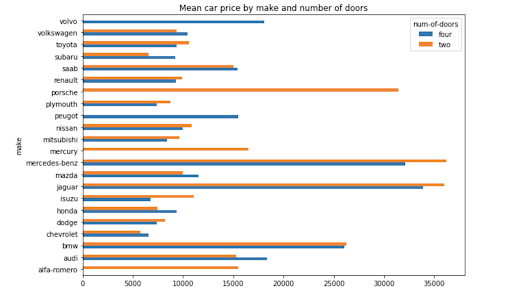

How to Calculate With Pandas Pivot Table

The aggfunc argument in the pivot table function can take in one or more standard calculations.

The following code calculates the mean and median price for car body style and the number of doors.

np.round(pd.pivot_table(data, values='price', index=['body-style'], columns=['num-of-doors'], aggfunc=[np.mean, np.median], fill_value=0),2)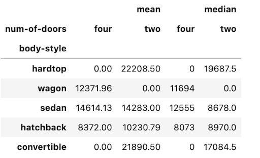

You can add the argument margins=True to add totals to columns and rows. You can also specify a name for the totals using margins_name .

np.round(pd.pivot_table(data, values='price', index=['body-style'], columns=['num-of-doors'], aggfunc=[np.sum], fill_value=0, margins=True, margins_name='Total'),2)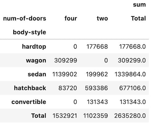

How to Style Your Pandas Pivot Table

When summarizing data, styling is important. We want to ensure that the patterns and insights that the pivot table is providing are easy to read and understand. In the pivot tables used in earlier parts of the article, very little styling has been applied. As a result, the tables are not easy to understand or visually appealing.

We can use another Pandas method, known as the style method to make the tables look prettier and easier to draw insights from. The code below adds appropriate formatting and units of measurement to each of the values used in this pivot table. It is now much easier to distinguish between the two columns and to comprehend what the data is telling you.

pivot = np.round(pd.pivot_table(data, values=['price', 'horsepower'], index=['make'], aggfunc=np.mean, fill_value=0),2) pivot.style.format(', 'horsepower':'hp'>)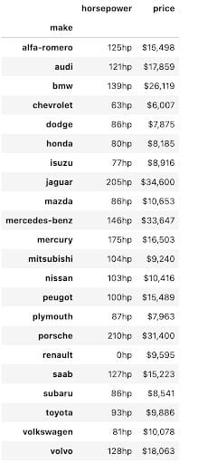

We can combine different formats using the styler and use the pandas built-in styles to summarize data in a way that instantly draws insights out. In the code and pivot table shown below, we have ordered the make of the car by price from high to low value, added appropriate formatting to the numbers and added a bar chart overlaying the values in both columns. This makes it easier to draw conclusions from the table, such as which make of car is the most expensive and how horsepower relates to the price for each car make.

pivot = np.round(pd.pivot_table(data, values=['price', 'horsepower'], index=['make'], aggfunc=np.mean, fill_value=0),2) pivot = pivot.reindex(pivot['price'].sort_values(ascending=False).index).nlargest(10, 'price') pivot.style.format(', 'horsepower':'hp'>).bar(color='#d65f5f')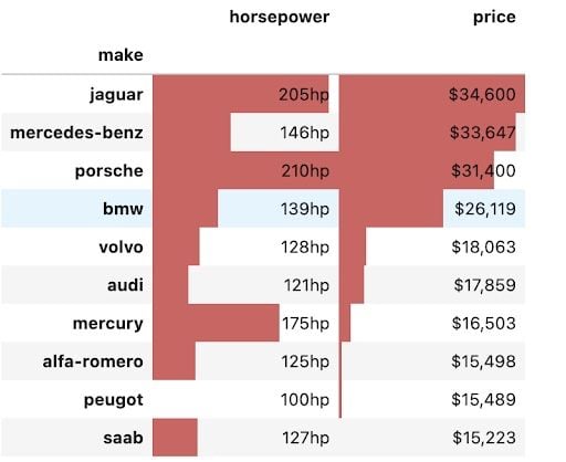

Advantages of Pandas Pivot Tables

Pivot tables have been in use since the early ’90s with Microsoft patenting the famous Excel version known as “PivotTable” in 1994. They are still widely used today because they are such a powerful tool for analyzing data. The Pandas pivot table brings this tool out of the spreadsheet and into the hands of Python users.

This guide gave a brief introduction to the usage of the pivot table tool in Pandas. It is meant to give a beginner a quick tutorial to get up and running with the tool but I suggest digging into the pandas documentation , which gives a more in-depth guide to this function.

Источник

Pivot Tables with Pandas

Most everyone who has worked with any type of data has likely used Microsoft Excel’s PivotTable function. It’s a quick, user-friendly tool that allows users to to calculate, aggregate, and summarize data sets enabling further analysis of patterns and trends. Excel provides an intuitive GUI that allows analysts to simply click, drag and drop data and easily apply whichever aggregation function they choose. It’s fantastic tool to use and aids when building Excel visualizations for business presentations.

Python’s Pandas library — which specializes in tabular data, similar to Excel — also has a .pivot_table() function that works in the same concept. It’s a powerful method, comes with a lot of customizable parameters, that should be in every analyst’s Python toolbox. It takes some time to understand the syntax behind the method, but once you’re familiar, it’s a lot faster and more efficient than Excel.

Let’s dive into an NBA stats dataset and see how Panda’s .pivot_table() function works!

#importing required libraries
import pandas as pd
import numpy as np#reading in the data & selecting needed columns
df = pd.read_csv('../Data/NBA_Player_seasonal.csv', index_col = 0)
df = df[['Player', 'Season', 'Age', 'Tm','WS', 'G','MP','3P','TRB','AST','STL','BLK', 'TOV', 'PF','PTS']]#displaying first 5 rows of dataframe
df.head()

Above, we can see a preview of our dataset. It’s seasonal totals for every NBA & ABA player dating back to the beginning of the league in 1947. It’s pre-sorted and ranked by highest “WS” — win-share, a metric that calculates the estimated number of wins a player contributes to their team. Let’s say we wanted to see this information, but aggregated by team. We could do something like this:

#creating a pivot table where team is the index
df.pivot_table(index = 'Tm')

By default, pivot_table() brings in all numerical columns and aggregates the data using it’s mean. Let’s say we only care about a few of these columns, and instead of the averages, we want to see totals.

#pivot table with selected columns & summed
df.pivot_table(df[['PTS', 'AST', 'TRB']], #selected columns 
index = 'Tm', #indexed by team 
aggfunc = np.sum) #aggregated by sum

Now we can view just the statistics we’re interested in and view totals instead of averages. You are able to pass in a library for the aggfunc argument, allowing users to choose which type of aggregation should be performed on each column.

Taking it a step further, pivot_table() allows users to have multiple indexes to further analyze data. Below is an example of the same data set but reshaped as teams statistics over the years.

#multi-index pivot table
df.pivot_table(df[['PTS', 'AST', 'TRB', 'STL','BLK', 'TOV']], 
index = ['Season', 'Tm'], 
aggfunc = np.mean).head()

In the above pivot table, we’re aggregating on missing data, even some of the basic statistics weren’t recorded until a few seasons after the inaugural one in 1947. Let’s say we want to fill those with zero’s for our analysis. We can accomplish this with a simple addition to our pivot table parameters.

#filling in NaN values w/ 0's
df.pivot_table(df[['PTS', 'AST', 'TRB', 'STL','BLK', 'TOV']], 
index = ['Season', 'Tm'], 
aggfunc = np.mean, 
fill_value = 0).head()

This function also enables users to quickly visualize their data in fewer lines of code, than if they were trying to code it directly from the original data set. As an example, let’s plot league-wide seasonal averages over the years via a pivot table line plot.

#plotting pivot table
df.pivot_table(df[['PTS', 'AST', 'TRB', 'STL','BLK', 'TOV']], 
index = ['Season',], 
aggfunc = np.mean, 
fill_value = 0).plot()

It’s not the prettiest visual, but it’s quick and provides some vital information. You can quickly identity the 1999 lockout seasons where only 50 games were played in the season compared to the usual 82.

These are several of the pivot_table() parameters you can use to customize/reshape your dataset. There are other parameters such as margins which adds totals to columns and rows. Another is columns which provides an additional way to segment your data set. Lastly, each pivot table outputs a new dataframe, that allows you to perform any standard dataframe functions/methods such as filtering on specific criteria, for example if we had only wanted to see Boston Celtics data.

I hope this quick tutorial is helpful to understand how powerful Panda’s pivot table function is! Please feel free to reach out with any questions or leave any feedback.

References

Источник