Pie charts in python

Plotly is a free and open-source graphing library for Python. We recommend you read our Getting Started guide for the latest installation or upgrade instructions, then move on to our Plotly Fundamentals tutorials or dive straight in to some Basic Charts tutorials.

A pie chart is a circular statistical chart, which is divided into sectors to illustrate numerical proportion.

If you’re looking instead for a multilevel hierarchical pie-like chart, go to the Sunburst tutorial.

Pie chart with plotly express¶

In px.pie , data visualized by the sectors of the pie is set in values . The sector labels are set in names .

import plotly.express as px df = px.data.gapminder().query("year == 2007").query("continent == 'Europe'") df.loc[df['pop']  2.e6, 'country'] = 'Other countries' # Represent only large countries fig = px.pie(df, values='pop', names='country', title='Population of European continent') fig.show()

Pie chart with repeated labels¶

Lines of the dataframe with the same value for names are grouped together in the same sector.

import plotly.express as px # This dataframe has 244 lines, but 4 distinct values for `day` df = px.data.tips() fig = px.pie(df, values='tip', names='day') fig.show()

Pie chart in Dash¶

Dash is the best way to build analytical apps in Python using Plotly figures. To run the app below, run pip install dash , click «Download» to get the code and run python app.py .

Get started with the official Dash docs and learn how to effortlessly style & deploy apps like this with Dash Enterprise.

Sign up for Dash Club → Free cheat sheets plus updates from Chris Parmer and Adam Schroeder delivered to your inbox every two months. Includes tips and tricks, community apps, and deep dives into the Dash architecture. Join now.

Setting the color of pie sectors with px.pie¶

import plotly.express as px df = px.data.tips() fig = px.pie(df, values='tip', names='day', color_discrete_sequence=px.colors.sequential.RdBu) fig.show()

Using an explicit mapping for discrete colors¶

For more information about discrete colors, see the dedicated page.

import plotly.express as px df = px.data.tips() fig = px.pie(df, values='tip', names='day', color='day', color_discrete_map='Thur':'lightcyan', 'Fri':'cyan', 'Sat':'royalblue', 'Sun':'darkblue'>) fig.show()

Customizing a pie chart created with px.pie¶

In the example below, we first create a pie chart with px,pie , using some of its options such as hover_data (which columns should appear in the hover) or labels (renaming column names). For further tuning, we call fig.update_traces to set other parameters of the chart (you can also use fig.update_layout for changing the layout).

import plotly.express as px df = px.data.gapminder().query("year == 2007").query("continent == 'Americas'") fig = px.pie(df, values='pop', names='country', title='Population of American continent', hover_data=['lifeExp'], labels='lifeExp':'life expectancy'>) fig.update_traces(textposition='inside', textinfo='percent+label') fig.show()

Basic Pie Chart with go.Pie¶

If Plotly Express does not provide a good starting point, it is also possible to use the more generic go.Pie class from plotly.graph_objects .

In go.Pie , data visualized by the sectors of the pie is set in values . The sector labels are set in labels . The sector colors are set in marker.colors .

If you’re looking instead for a multilevel hierarchical pie-like chart, go to the Sunburst tutorial.

import plotly.graph_objects as go labels = ['Oxygen','Hydrogen','Carbon_Dioxide','Nitrogen'] values = [4500, 2500, 1053, 500] fig = go.Figure(data=[go.Pie(labels=labels, values=values)]) fig.show()

Styled Pie Chart¶

Colors can be given as RGB triplets or hexadecimal strings, or with CSS color names as below.

import plotly.graph_objects as go colors = ['gold', 'mediumturquoise', 'darkorange', 'lightgreen'] fig = go.Figure(data=[go.Pie(labels=['Oxygen','Hydrogen','Carbon_Dioxide','Nitrogen'], values=[4500,2500,1053,500])]) fig.update_traces(hoverinfo='label+percent', textinfo='value', textfont_size=20, marker=dict(colors=colors, line=dict(color='#000000', width=2))) fig.show()

Controlling text fontsize with uniformtext¶

If you want all the text labels to have the same size, you can use the uniformtext layout parameter. The minsize attribute sets the font size, and the mode attribute sets what happens for labels which cannot fit with the desired fontsize: either hide them or show them with overflow. In the example below we also force the text to be inside with textposition , otherwise text labels which do not fit are displayed outside of pie sectors.

import plotly.express as px df = px.data.gapminder().query("continent == 'Asia'") fig = px.pie(df, values='pop', names='country') fig.update_traces(textposition='inside') fig.update_layout(uniformtext_minsize=12, uniformtext_mode='hide') fig.show()

Controlling text orientation inside pie sectors¶

The insidetextorientation attribute controls the orientation of text inside sectors. With «auto» the texts may automatically be rotated to fit with the maximum size inside the slice. Using «horizontal» (resp. «radial», «tangential») forces text to be horizontal (resp. radial or tangential)

For a figure fig created with plotly express, use fig.update_traces(insidetextorientation=’. ‘) to change the text orientation.

import plotly.graph_objects as go labels = ['Oxygen','Hydrogen','Carbon_Dioxide','Nitrogen'] values = [4500, 2500, 1053, 500] fig = go.Figure(data=[go.Pie(labels=labels, values=values, textinfo='label+percent', insidetextorientation='radial' )]) fig.show()

Donut Chart¶

import plotly.graph_objects as go labels = ['Oxygen','Hydrogen','Carbon_Dioxide','Nitrogen'] values = [4500, 2500, 1053, 500] # Use `hole` to create a donut-like pie chart fig = go.Figure(data=[go.Pie(labels=labels, values=values, hole=.3)]) fig.show()

Pulling sectors out from the center¶

For a «pulled-out» or «exploded» layout of the pie chart, use the pull argument. It can be a scalar for pulling all sectors or an array to pull only some of the sectors.

import plotly.graph_objects as go labels = ['Oxygen','Hydrogen','Carbon_Dioxide','Nitrogen'] values = [4500, 2500, 1053, 500] # pull is given as a fraction of the pie radius fig = go.Figure(data=[go.Pie(labels=labels, values=values, pull=[0, 0, 0.2, 0])]) fig.show()

Pie Charts in subplots¶

import plotly.graph_objects as go from plotly.subplots import make_subplots labels = ["US", "China", "European Union", "Russian Federation", "Brazil", "India", "Rest of World"] # Create subplots: use 'domain' type for Pie subplot fig = make_subplots(rows=1, cols=2, specs=[['type':'domain'>, 'type':'domain'>]]) fig.add_trace(go.Pie(labels=labels, values=[16, 15, 12, 6, 5, 4, 42], name="GHG Emissions"), 1, 1) fig.add_trace(go.Pie(labels=labels, values=[27, 11, 25, 8, 1, 3, 25], name="CO2 Emissions"), 1, 2) # Use `hole` to create a donut-like pie chart fig.update_traces(hole=.4, hoverinfo="label+percent+name") fig.update_layout( title_text="Global Emissions 1990-2011", # Add annotations in the center of the donut pies. annotations=[dict(text='GHG', x=0.18, y=0.5, font_size=20, showarrow=False), dict(text='CO2', x=0.82, y=0.5, font_size=20, showarrow=False)]) fig.show()

import plotly.graph_objects as go from plotly.subplots import make_subplots labels = ['1st', '2nd', '3rd', '4th', '5th'] # Define color sets of paintings night_colors = ['rgb(56, 75, 126)', 'rgb(18, 36, 37)', 'rgb(34, 53, 101)', 'rgb(36, 55, 57)', 'rgb(6, 4, 4)'] sunflowers_colors = ['rgb(177, 127, 38)', 'rgb(205, 152, 36)', 'rgb(99, 79, 37)', 'rgb(129, 180, 179)', 'rgb(124, 103, 37)'] irises_colors = ['rgb(33, 75, 99)', 'rgb(79, 129, 102)', 'rgb(151, 179, 100)', 'rgb(175, 49, 35)', 'rgb(36, 73, 147)'] cafe_colors = ['rgb(146, 123, 21)', 'rgb(177, 180, 34)', 'rgb(206, 206, 40)', 'rgb(175, 51, 21)', 'rgb(35, 36, 21)'] # Create subplots, using 'domain' type for pie charts specs = [['type':'domain'>, 'type':'domain'>], ['type':'domain'>, 'type':'domain'>]] fig = make_subplots(rows=2, cols=2, specs=specs) # Define pie charts fig.add_trace(go.Pie(labels=labels, values=[38, 27, 18, 10, 7], name='Starry Night', marker_colors=night_colors), 1, 1) fig.add_trace(go.Pie(labels=labels, values=[28, 26, 21, 15, 10], name='Sunflowers', marker_colors=sunflowers_colors), 1, 2) fig.add_trace(go.Pie(labels=labels, values=[38, 19, 16, 14, 13], name='Irises', marker_colors=irises_colors), 2, 1) fig.add_trace(go.Pie(labels=labels, values=[31, 24, 19, 18, 8], name='The Night Café', marker_colors=cafe_colors), 2, 2) # Tune layout and hover info fig.update_traces(hoverinfo='label+percent+name', textinfo='none') fig.update(layout_title_text='Van Gogh: 5 Most Prominent Colors Shown Proportionally', layout_showlegend=False) fig = go.Figure(fig) fig.show()

Plot chart with area proportional to total count¶

Plots in the same scalegroup are represented with an area proportional to their total size.

import plotly.graph_objects as go from plotly.subplots import make_subplots labels = ["Asia", "Europe", "Africa", "Americas", "Oceania"] fig = make_subplots(1, 2, specs=[['type':'domain'>, 'type':'domain'>]], subplot_titles=['1980', '2007']) fig.add_trace(go.Pie(labels=labels, values=[4, 7, 1, 7, 0.5], scalegroup='one', name="World GDP 1980"), 1, 1) fig.add_trace(go.Pie(labels=labels, values=[21, 15, 3, 19, 1], scalegroup='one', name="World GDP 2007"), 1, 2) fig.update_layout(title_text='World GDP') fig.show()

Источник

Matplotlib Pie Charts

With Pyplot, you can use the pie() function to draw pie charts:

Example

import matplotlib.pyplot as plt
import numpy as np

Result:

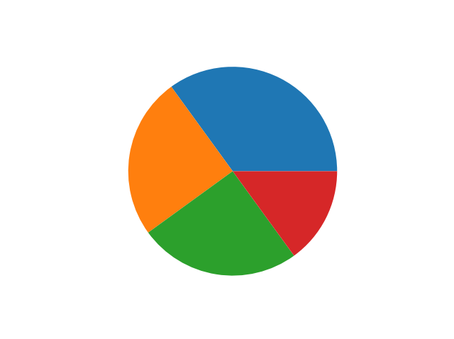
As you can see the pie chart draws one piece (called a wedge) for each value in the array (in this case [35, 25, 25, 15]).

By default the plotting of the first wedge starts from the x-axis and moves counterclockwise:

Note: The size of each wedge is determined by comparing the value with all the other values, by using this formula:

The value divided by the sum of all values: x/sum(x)

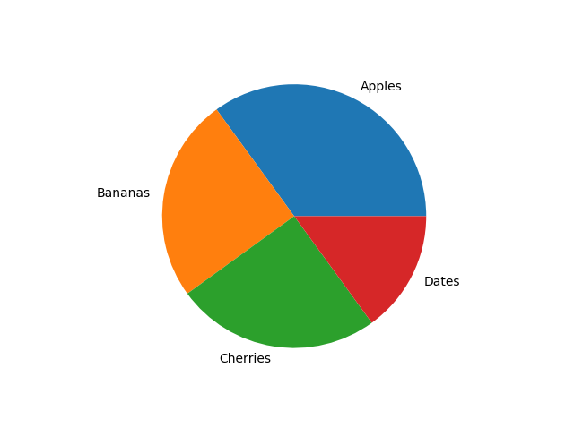
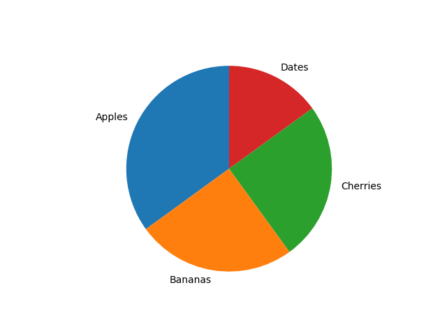
Labels

Add labels to the pie chart with the label parameter.

The label parameter must be an array with one label for each wedge:

Example

import matplotlib.pyplot as plt
import numpy as np

y = np.array([35, 25, 25, 15])
mylabels = [«Apples», «Bananas», «Cherries», «Dates»]

plt.pie(y, labels = mylabels)
plt.show()

Result:

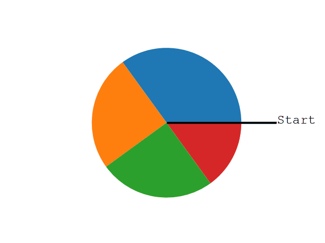
Start Angle

As mentioned the default start angle is at the x-axis, but you can change the start angle by specifying a startangle parameter.

The startangle parameter is defined with an angle in degrees, default angle is 0:

Example

Start the first wedge at 90 degrees:

import matplotlib.pyplot as plt
import numpy as np

y = np.array([35, 25, 25, 15])
mylabels = [«Apples», «Bananas», «Cherries», «Dates»]

plt.pie(y, labels = mylabels, startangle = 90)
plt.show()

Result:

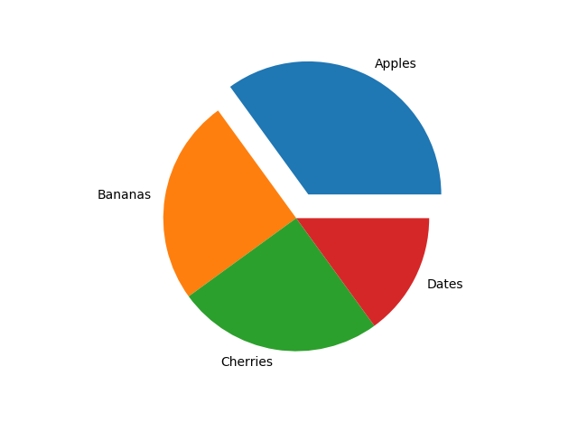
Explode

Maybe you want one of the wedges to stand out? The explode parameter allows you to do that.

The explode parameter, if specified, and not None , must be an array with one value for each wedge.

Each value represents how far from the center each wedge is displayed:

Example

Pull the «Apples» wedge 0.2 from the center of the pie:

import matplotlib.pyplot as plt
import numpy as np

y = np.array([35, 25, 25, 15])
mylabels = [«Apples», «Bananas», «Cherries», «Dates»]
myexplode = [0.2, 0, 0, 0]

plt.pie(y, labels = mylabels, explode = myexplode)
plt.show()

Result:

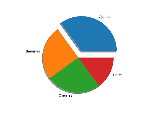
Shadow

Add a shadow to the pie chart by setting the shadows parameter to True :

Example

import matplotlib.pyplot as plt
import numpy as np

y = np.array([35, 25, 25, 15])
mylabels = [«Apples», «Bananas», «Cherries», «Dates»]
myexplode = [0.2, 0, 0, 0]

plt.pie(y, labels = mylabels, explode = myexplode, shadow = True)
plt.show()

Result:

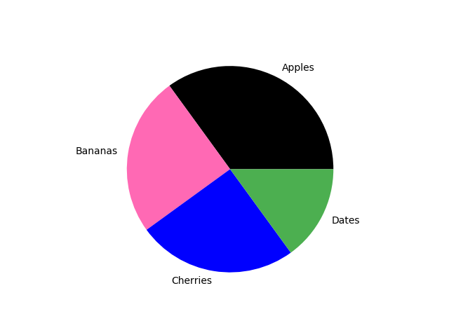
Colors

You can set the color of each wedge with the colors parameter.

The colors parameter, if specified, must be an array with one value for each wedge:

Example

Specify a new color for each wedge:

import matplotlib.pyplot as plt
import numpy as np

y = np.array([35, 25, 25, 15])
mylabels = [«Apples», «Bananas», «Cherries», «Dates»]
mycolors = [«black», «hotpink», «b», «#4CAF50»]

plt.pie(y, labels = mylabels, colors = mycolors)
plt.show()

Result:

You can use Hexadecimal color values, any of the 140 supported color names, or one of these shortcuts:

‘r’ — Red
‘g’ — Green
‘b’ — Blue
‘c’ — Cyan
‘m’ — Magenta
‘y’ — Yellow
‘k’ — Black
‘w’ — White

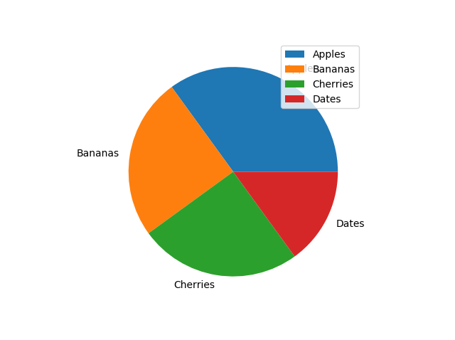
Legend

To add a list of explanation for each wedge, use the legend() function:

Example

import matplotlib.pyplot as plt
import numpy as np

y = np.array([35, 25, 25, 15])
mylabels = [«Apples», «Bananas», «Cherries», «Dates»]

plt.pie(y, labels = mylabels)
plt.legend()
plt.show()

Result:

Legend With Header

To add a header to the legend, add the title parameter to the legend function.

Example

Add a legend with a header:

import matplotlib.pyplot as plt
import numpy as np

y = np.array([35, 25, 25, 15])
mylabels = [«Apples», «Bananas», «Cherries», «Dates»]

plt.pie(y, labels = mylabels)
plt.legend(title = «Four Fruits:»)
plt.show()

Источник

Pie charts in python