Opencv pose estimation python

Deep Learning based Human Pose Estimation using OpenCV

In this tutorial, Deep Learning based Human Pose Estimation using OpenCV. We will explain in detail how to use a pre-trained Caffe model that won the COCO keypoints challenge in 2016 in your own application. We will briefly go over the architecture to get an idea of what is going on under the hood.

1. Pose Estimation (a.k.a Keypoint Detection)

Pose Estimation is a general problem in Computer Vision where we detect the position and orientation of an object. This usually means detecting keypoint locations that describe the object.

For example, in the problem of face pose estimation (a.k.a facial landmark detection), we detect landmarks on a human face. We have written extensively on the topic. Please see our articles on ( Facial Landmark Detection using OpenCV and Facial Landmark Detection using Dlib )

A related problem is Head Pose Estimation where we use the facial landmarks to obtain the 3D orientation of a human head with respect to the camera.

In this article, we will focus on human pose estimation, where it is required to detect and localize the major parts/joints of the body ( e.g. shoulders, ankle, knee, wrist etc. ).

Remember the scene where Tony stark wears the Iron Man suit using gestures?

If such a suit is ever built, it would require human pose estimation!

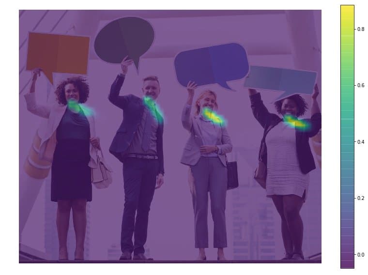
For the purpose of this article, though, we will tone down our ambition a tiny bit and solve a simpler problem of detecting keypoints on the body. A typical output of a pose detector looks as shown below :

1.1. Keypoint Detection Datasets

Until recently, there was little progress in pose estimation because of the lack of high-quality datasets. Such is the enthusiasm in AI these days that people believe every problem is just a good dataset away from being demolished. Some challenging datasets have been released in the last few years which have made it easier for researchers to attack the problem with all their intellectual might.

If we missed an important dataset, please mention in the comments and we will be happy to include in this list!

2. Multi-Person Pose Estimation model

The model used in this tutorial is based on a paper titled Multi-Person Pose Estimation by the Perceptual Computing Lab at Carnegie Mellon University. The authors of the paper train a very deep Neural Networks for this task. Let’s briefly go over the architecture before we explain how to use the pre-trained model.

2.1. Architecture Overview

The model takes as input a color image of size w × h and produces, as output, the 2D locations of keypoints for each person in the image. The detection takes place in three stages :

1. Stage 0: The first 10 layers of the VGGNet are used to create feature maps for the input image.
2. Stage 1: A 2-branch multi-stage CNN is used where the first branch predicts a set of 2D confidence maps (S) of body part locations ( e.g. elbow, knee etc.). Given below are confidence maps and Affinity maps for the keypoint – Left Shoulder.

The second branch predicts a set of 2D vector fields (L) of part affinities, which encode the degree of association between parts. In the figure below part affinity between the Neck and Left shoulder is shown.

Stage 2: The confidence and affinity maps are parsed by greedy inference to produce the 2D keypoints for all people in the image.

This architecture won the COCO keypoints challenge in 2016.

2.2 Pre-trained models for Human Pose Estimation

The authors of the paper have shared two models – one is trained on the Multi-Person Dataset ( MPII ) and the other is trained on the COCO dataset. The COCO model produces 18 points, while the MPII model outputs 15 points. The outputs plotted on a person is shown in the image below.

COCO Output Format Nose – 0, Neck – 1, Right Shoulder – 2, Right Elbow – 3, Right Wrist – 4, Left Shoulder – 5, Left Elbow – 6, Left Wrist – 7, Right Hip – 8, Right Knee – 9, Right Ankle – 10, Left Hip – 11, Left Knee – 12, LAnkle – 13, Right Eye – 14, Left Eye – 15, Right Ear – 16, Left Ear – 17, Background – 18 MPII Output Format Head – 0, Neck – 1, Right Shoulder – 2, Right Elbow – 3, Right Wrist – 4, Left Shoulder – 5, Left Elbow – 6, Left Wrist – 7, Right Hip – 8, Right Knee – 9, Right Ankle – 10, Left Hip – 11, Left Knee – 12, Left Ankle – 13, Chest – 14, Background – 15

You can download the model weight files using the scripts provided at this location.

3. Code for Human Pose Estimation in OpenCV

In this section, we will see how to load the trained models in OpenCV and check the outputs. We will discuss code for only single person pose estimation to keep things simple. As we saw in the previous section that the output consists of confidence maps and affinity maps. These outputs can be used to find the pose for every person in a frame if multiple people are present. We will cover the multiple-person case in a future post.

First, download the code and model files from below. There are separate files for Image and Video inputs. Please go through the README file if you encounter any difficulty in running the code.

3.1. Step 1 : Download Model Weights

Use the getModels.sh file provided with the code to download all the model weights to the respective folders. Note that the configuration proto files are already present in the folders.

From the command line, execute the following from the downloaded folder.

sudo chmod a+x getModels.sh ./getModels.sh

Check the folders to ensure that the model binaries (.caffemodel files ) have been downloaded. If you are not able to run the above script, then you can download the model by clicking here for the MPII model and here for COCO model.

3.2 Step 2: Load Network

We are using models trained on Caffe Deep Learning Framework. Caffe models have 2 files –

1. .prototxt file which specifies the architecture of the neural network – how the different layers are arranged etc.
2. .caffemodel file which stores the weights of the trained model

We will use these two files to load the network into memory.

Download Code To easily follow along this tutorial, please download code by clicking on the button below. It’s FREE!

// Specify the paths for the 2 files string protoFile = "pose/mpi/pose_deploy_linevec_faster_4_stages.prototxt"; string weightsFile = "pose/mpi/pose_iter_160000.caffemodel"; // Read the network into Memory Net net = readNetFromCaffe(protoFile, weightsFile);

# Specify the paths for the 2 files protoFile = "pose/mpi/pose_deploy_linevec_faster_4_stages.prototxt" weightsFile = "pose/mpi/pose_iter_160000.caffemodel" # Read the network into Memory net = cv2.dnn.readNetFromCaffe(protoFile, weightsFile)

3.3. Step 3: Read Image and Prepare Input to the Network

The input frame that we read using OpenCV should be converted to a input blob ( like Caffe ) so that it can be fed to the network. This is done using the blobFromImage function which converts the image from OpenCV format to Caffe blob format. The parameters are to be provided in the blobFromImage function. First we normalize the pixel values to be in (0,1). Then we specify the dimensions of the image. Next, the Mean value to be subtracted, which is (0,0,0). There is no need to swap the R and B channels since both OpenCV and Caffe use BGR format.
C++

// Mat frame = imread("single.jpg"); // Specify the input image dimensions int inWidth = 368; int inHeight = 368; // Prepare the frame to be fed to the network Mat inpBlob = blobFromImage(frame, 1.0 / 255, Size(inWidth, inHeight), Scalar(0, 0, 0), false, false); // Set the prepared object as the input blob of the network net.setInput(inpBlob);

# Read image frame = cv2.imread("single.jpg") # Specify the input image dimensions inWidth = 368 inHeight = 368 # Prepare the frame to be fed to the network inpBlob = cv2.dnn.blobFromImage(frame, 1.0 / 255, (inWidth, inHeight), (0, 0, 0), swapRB=False, crop=False) # Set the prepared object as the input blob of the network net.setInput(inpBlob)

3.4. Step 4: Make Predictions and Parse Keypoints

Once the image is passed to the model, the predictions can be made using a single line of code. The forward method for the DNN class in OpenCV makes a forward pass through the network which is just another way of saying it is making a prediction.

The output is a 4D matrix :

1. The first dimension being the image ID ( in case you pass more than one image to the network ).
2. The second dimension indicates the index of a keypoint. The model produces Confidence Maps and Part Affinity maps which are all concatenated. For COCO model it consists of 57 parts – 18 keypoint confidence Maps + 1 background + 19*2 Part Affinity Maps. Similarly, for MPI, it produces 44 points. We will be using only the first few points which correspond to Keypoints.
3. The third dimension is the height of the output map.
4. The fourth dimension is the width of the output map.

We check whether each keypoint is present in the image or not. We get the location of the keypoint by finding the maxima of the confidence map of that keypoint. We also use a threshold to reduce false detections.

Once the keypoints are detected, we just plot them on the image.
C++

int H = output.size[2]; int W = output.size[3]; // find the position of the body parts vector points(nPoints); for (int n=0; n < nPoints; n++) < // Probability map of corresponding body's part. Mat probMap(H, W, CV_32F, output.ptr(0,n)); Point2f p(-1,-1); Point maxLoc; double prob; minMaxLoc(probMap, 0, &prob, 0, &maxLoc); if (prob >thresh) < p = maxLoc; p.x *= (float)frameWidth / W ; p.y *= (float)frameHeight / H ; circle(frameCopy, cv::Point((int)p.x, (int)p.y), 8, Scalar(0,255,255), -1); cv::putText(frameCopy, cv::format("%d", n), cv::Point((int)p.x, (int)p.y), cv::FONT_HERSHEY_COMPLEX, 1, cv::Scalar(0, 0, 255), 2); >points[n] = p; >

H = out.shape[2] W = out.shape[3] # Empty list to store the detected keypoints points = [] for i in range(len()): # confidence map of corresponding body's part. probMap = output[0, i, :, :] # Find global maxima of the probMap. minVal, prob, minLoc, point = cv2.minMaxLoc(probMap) # Scale the point to fit on the original image x = (frameWidth * point[0]) / W y = (frameHeight * point[1]) / H if prob > threshold : cv2.circle(frame, (int(x), int(y)), 15, (0, 255, 255), thickness=-1, lineType=cv.FILLED) cv2.putText(frame, "<>".format(i), (int(x), int(y)), cv2.FONT_HERSHEY_SIMPLEX, 1.4, (0, 0, 255), 3, lineType=cv2.LINE_AA) # Add the point to the list if the probability is greater than the threshold points.append((int(x), int(y))) else : points.append(None) cv2.imshow("Output-Keypoints",frame) cv2.waitKey(0) cv2.destroyAllWindows()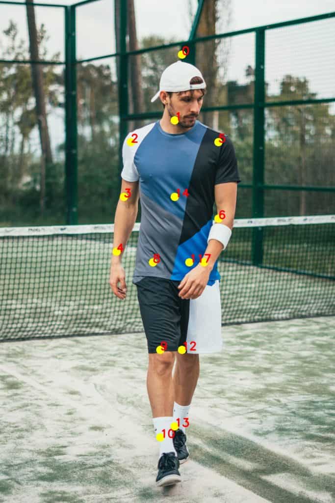

3.5. Step 5: Draw Skeleton

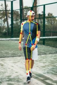
Since we know the indices of the points before-hand, we can draw the skeleton when we have the keypoints by just joining the pairs. This is done using the code given below.

for (int n = 0; n < nPairs; n++) < // lookup 2 connected body/hand parts Point2f partA = points[POSE_PAIRS[n][0]]; Point2f partB = points[POSE_PAIRS[n][1]]; if (partA.x

for pair in POSE_PAIRS: partA = pair[0] partB = pair[1] if points[partA] and points[partB]: cv2.line(frameCopy, points[partA], points[partB], (0, 255, 0), 3)

Do checkout the Video demo using the video version of the code. We found that COCO model is 1.5 times slower than the MPI model. This is expected as we are using a stripped down version having 4 stages.

If you have ideas of some cool applications using these methods, do mention them in the comments!

Subscribe & Download Code

If you liked this article and would like to download code (C++ and Python) and example images used in this post, please click here. Alternately, sign up to receive a free Computer Vision Resource Guide. In our newsletter, we share OpenCV tutorials and examples written in C++/Python, and Computer Vision and Machine Learning algorithms and news.

Источник