Python OpenCV: Optical Flow with Lucas-Kanade method
OpenCV is a huge open-source library for computer vision, machine learning, and image processing. OpenCV supports a wide variety of programming languages like Python, C++, Java, etc. It can process images and videos to identify objects, faces, or even the handwriting of a human. When it is integrated with various libraries, such as Numpy which is a highly optimized library for numerical operations, then the number of weapons increases in your Arsenal i.e whatever operations one can do in Numpy can be combined with OpenCV.
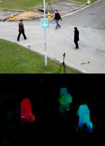
In this article, we will be learning how to apply the Lucas-Kanade method to track some points on a video. To track the points, first, we need to find the points to be tracked. For finding the points, we’ll use cv2.goodFeaturesToTrack() . Now, we will capture the first frame and detect some corner points. These points will be tracked using the Lucas-Kanade Algorithm provided by OpenCV, i.e, cv2.calcOpticalFlowPyrLK() .
Syntax: cv2.calcOpticalFlowPyrLK(prevImg, nextImg, prevPts, nextPts[, winSize[, maxLevel[, criteria]]])
Parameters:
prevImg – first 8-bit input image
nextImg – second input image
prevPts – vector of 2D points for which the flow needs to be found.
winSize – size of the search window at each pyramid level.
maxLevel – 0-based maximal pyramid level number; if set to 0, pyramids are not used (single level), if set to 1, two levels are used, and so on.
criteria – parameter, specifying the termination criteria of the iterative search algorithm.
Return:
nextPts – output vector of 2D points (with single-precision floating-point coordinates) containing the calculated new positions of input features in the second image; when OPTFLOW_USE_INITIAL_FLOW flag is passed, the vector must have the same size as in the input.
status – output status vector (of unsigned chars); each element of the vector is set to 1 if the flow for the corresponding features has been found, otherwise, it is set to 0.
err – output vector of errors; each element of the vector is set to an error for the corresponding feature, type of the error measure can be set in flags parameter; if the flow wasn’t found then the error is not defined (use the status parameter to find such cases).
Opencv optical flow python
- We will understand the concepts of optical flow and its estimation using Lucas-Kanade method.
- We will use functions like cv2.calcOpticalFlowPyrLK() to track feature points in a video.
Optical Flow
Optical flow is the pattern of apparent motion of image objects between two consecutive frames caused by the movemement of object or camera. It is 2D vector field where each vector is a displacement vector showing the movement of points from first frame to second. Consider the image below (Image Courtesy: Wikipedia article on Optical Flow).

It shows a ball moving in 5 consecutive frames. The arrow shows its displacement vector. Optical flow has many applications in areas like :
Optical flow works on several assumptions:
- The pixel intensities of an object do not change between consecutive frames.
- Neighbouring pixels have similar motion.
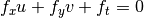
Consider a pixel \(I(x,y,t)\) in first frame (Check a new dimension, time, is added here. Earlier we were working with images only, so no need of time). It moves by distance \((dx,dy)\) in next frame taken after \(dt\) time. So since those pixels are the same and intensity does not change, we can say,
Then take taylor series approximation of right-hand side, remove common terms and divide by \(dt\) to get the following equation:
Above equation is called Optical Flow equation. In it, we can find \(f_x\) and \(f_y\), they are image gradients. Similarly \(f_t\) is the gradient along time. But \((u,v)\) is unknown. We cannot solve this one equation with two unknown variables. So several methods are provided to solve this problem and one of them is Lucas-Kanade.
Lucas-Kanade method
We have seen an assumption before, that all the neighbouring pixels will have similar motion. Lucas-Kanade method takes a 3×3 patch around the point. So all the 9 points have the same motion. We can find \((f_x, f_y, f_t)\) for these 9 points. So now our problem becomes solving 9 equations with two unknown variables which is over-determined. A better solution is obtained with least square fit method. Below is the final solution which is two equation-two unknown problem and solve to get the solution.
( Check similarity of inverse matrix with Harris corner detector. It denotes that corners are better points to be tracked.)
So from user point of view, idea is simple, we give some points to track, we receive the optical flow vectors of those points. But again there are some problems. Until now, we were dealing with small motions. So it fails when there is large motion. So again we go for pyramids. When we go up in the pyramid, small motions are removed and large motions becomes small motions. So applying Lucas-Kanade there, we get optical flow along with the scale.
Lucas-Kanade Optical Flow in OpenCV
OpenCV provides all these in a single function, cv2.calcOpticalFlowPyrLK(). Here, we create a simple application which tracks some points in a video. To decide the points, we use cv2.goodFeaturesToTrack(). We take the first frame, detect some Shi-Tomasi corner points in it, then we iteratively track those points using Lucas-Kanade optical flow. For the function cv2.calcOpticalFlowPyrLK() we pass the previous frame, previous points and next frame. It returns next points along with some status numbers which has a value of 1 if next point is found, else zero. We iteratively pass these next points as previous points in next step. See the code below:
Optical Flow
Optical flow is the pattern of apparent motion of image objects between two consecutive frames caused by the movemement of object or camera. It is 2D vector field where each vector is a displacement vector showing the movement of points from first frame to second. Consider the image below (Image Courtesy: Wikipedia article on Optical Flow).
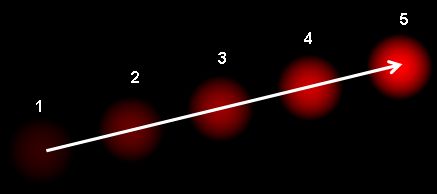
It shows a ball moving in 5 consecutive frames. The arrow shows its displacement vector. Optical flow has many applications in areas like :
Optical flow works on several assumptions:
- The pixel intensities of an object do not change between consecutive frames.
- Neighbouring pixels have similar motion.
Consider a pixel  in first frame (Check a new dimension, time, is added here. Earlier we were working with images only, so no need of time). It moves by distance
  in next frame taken after
  time. So since those pixels are the same and intensity does not change, we can say,

Then take taylor series approximation of right-hand side, remove common terms and divide by to get the following equation:


Lucas-Kanade method

We have seen an assumption before, that all the neighbouring pixels will have similar motion. Lucas-Kanade method takes a 3×3 patch around the point. So all the 9 points have the same motion. We can find for these 9 points. So now our problem becomes solving 9 equations with two unknown variables which is over-determined. A better solution is obtained with least square fit method. Below is the final solution which is two equation-two unknown problem and solve to get the solution.
![\begin</p></noscript><p> u \\ v \end = \begin \sum_>^2 & \sum_ f_ > \\ \sum_ f_> & \sum_<f_>^2 \end^ \begin — \sum_ f_> \\ — \sum_ <f_f_> \end»/></p><p>( Check similarity of inverse matrix with Harris corner detector. It denotes that corners are better points to be tracked.)</p><p>So from user point of view, idea is simple, we give some points to track, we receive the optical flow vectors of those points. But again there are some problems. Until now, we were dealing with small motions. So it fails when there is large motion. So again we go for pyramids. When we go up in the pyramid, small motions are removed and large motions becomes small motions. So applying Lucas-Kanade there, we get optical flow along with the scale.</p><h2>Lucas-Kanade Optical Flow in OpenCV¶</h2><p>OpenCV provides all these in a single function, <strong>cv2.calcOpticalFlowPyrLK()</strong>. Here, we create a simple application which tracks some points in a video. To decide the points, we use <strong>cv2.goodFeaturesToTrack()</strong>. We take the first frame, detect some Shi-Tomasi corner points in it, then we iteratively track those points using Lucas-Kanade optical flow. For the function <strong>cv2.calcOpticalFlowPyrLK()</strong> we pass the previous frame, previous points and next frame. It returns next points along with some status numbers which has a value of 1 if next point is found, else zero. We iteratively pass these next points as previous points in next step. See the code below:</p><pre><span >import</span> <span >numpy</span> <span >as</span> <span >np</span> <span >import</span> <span >cv2</span> <span >cap</span> <span >=</span> <span >cv2</span><span >.</span><span >VideoCapture</span><span >(</span><span >'slow.flv'</span><span >)</span> <span ># params for ShiTomasi corner detection</span> <span >feature_params</span> <span >=</span> <span >dict</span><span >(</span> <span >maxCorners</span> <span >=</span> <span >100</span><span >,</span> <span >qualityLevel</span> <span >=</span> <span >0.3</span><span >,</span> <span >minDistance</span> <span >=</span> <span >7</span><span >,</span> <span >blockSize</span> <span >=</span> <span >7</span> <span >)</span> <span ># Parameters for lucas kanade optical flow</span> <span >lk_params</span> <span >=</span> <span >dict</span><span >(</span> <span >winSize</span> <span >=</span> <span >(</span><span >15</span><span >,</span><span >15</span><span >),</span> <span >maxLevel</span> <span >=</span> <span >2</span><span >,</span> <span >criteria</span> <span >=</span> <span >(</span><span >cv2</span><span >.</span><span >TERM_CRITERIA_EPS</span> <span >|</span> <span >cv2</span><span >.</span><span >TERM_CRITERIA_COUNT</span><span >,</span> <span >10</span><span >,</span> <span >0.03</span><span >))</span> <span ># Create some random colors</span> <span >color</span> <span >=</span> <span >np</span><span >.</span><span >random</span><span >.</span><span >randint</span><span >(</span><span >0</span><span >,</span><span >255</span><span >,(</span><span >100</span><span >,</span><span >3</span><span >))</span> <span ># Take first frame and find corners in it</span> <span >ret</span><span >,</span> <span >old_frame</span> <span >=</span> <span >cap</span><span >.</span><span >read</span><span >()</span> <span >old_gray</span> <span >=</span> <span >cv2</span><span >.</span><span >cvtColor</span><span >(</span><span >old_frame</span><span >,</span> <span >cv2</span><span >.</span><span >COLOR_BGR2GRAY</span><span >)</span> <span >p0</span> <span >=</span> <span >cv2</span><span >.</span><span >goodFeaturesToTrack</span><span >(</span><span >old_gray</span><span >,</span> <span >mask</span> <span >=</span> <span >None</span><span >,</span> <span >**</span><span >feature_params</span><span >)</span> <span ># Create a mask image for drawing purposes</span> <span >mask</span> <span >=</span> <span >np</span><span >.</span><span >zeros_like</span><span >(</span><span >old_frame</span><span >)</span> <span >while</span><span >(</span><span >1</span><span >):</span> <span >ret</span><span >,</span><span >frame</span> <span >=</span> <span >cap</span><span >.</span><span >read</span><span >()</span> <span >frame_gray</span> <span >=</span> <span >cv2</span><span >.</span><span >cvtColor</span><span >(</span><span >frame</span><span >,</span> <span >cv2</span><span >.</span><span >COLOR_BGR2GRAY</span><span >)</span> <span ># calculate optical flow</span> <span >p1</span><span >,</span> <span >st</span><span >,</span> <span >err</span> <span >=</span> <span >cv2</span><span >.</span><span >calcOpticalFlowPyrLK</span><span >(</span><span >old_gray</span><span >,</span> <span >frame_gray</span><span >,</span> <span >p0</span><span >,</span> <span >None</span><span >,</span> <span >**</span><span >lk_params</span><span >)</span> <span ># Select good points</span> <span >good_new</span> <span >=</span> <span >p1</span><span >[</span><span >st</span><span >==</span><span >1</span><span >]</span> <span >good_old</span> <span >=</span> <span >p0</span><span >[</span><span >st</span><span >==</span><span >1</span><span >]</span> <span ># draw the tracks</span> <span >for</span> <span >i</span><span >,(</span><span >new</span><span >,</span><span >old</span><span >)</span> <span >in</span> <span >enumerate</span><span >(</span><span >zip</span><span >(</span><span >good_new</span><span >,</span><span >good_old</span><span >)):</span> <span >a</span><span >,</span><span >b</span> <span >=</span> <span >new</span><span >.</span><span >ravel</span><span >()</span> <span >c</span><span >,</span><span >d</span> <span >=</span> <span >old</span><span >.</span><span >ravel</span><span >()</span> <span >mask</span> <span >=</span> <span >cv2</span><span >.</span><span >line</span><span >(</span><span >mask</span><span >,</span> <span >(</span><span >a</span><span >,</span><span >b</span><span >),(</span><span >c</span><span >,</span><span >d</span><span >),</span> <span >color</span><span >[</span><span >i</span><span >]</span><span >.</span><span >tolist</span><span >(),</span> <span >2</span><span >)</span> <span >frame</span> <span >=</span> <span >cv2</span><span >.</span><span >circle</span><span >(</span><span >frame</span><span >,(</span><span >a</span><span >,</span><span >b</span><span >),</span><span >5</span><span >,</span><span >color</span><span >[</span><span >i</span><span >]</span><span >.</span><span >tolist</span><span >(),</span><span >-</span><span >1</span><span >)</span> <span >img</span> <span >=</span> <span >cv2</span><span >.</span><span >add</span><span >(</span><span >frame</span><span >,</span><span >mask</span><span >)</span> <span >cv2</span><span >.</span><span >imshow</span><span >(</span><span >'frame'</span><span >,</span><span >img</span><span >)</span> <span >k</span> <span >=</span> <span >cv2</span><span >.</span><span >waitKey</span><span >(</span><span >30</span><span >)</span> <span >&</span> <span >0xff</span> <span >if</span> <span >k</span> <span >==</span> <span >27</span><span >:</span> <span >break</span> <span ># Now update the previous frame and previous points</span> <span >old_gray</span> <span >=</span> <span >frame_gray</span><span >.</span><span >copy</span><span >()</span> <span >p0</span> <span >=</span> <span >good_new</span><span >.</span><span >reshape</span><span >(</span><span >-</span><span >1</span><span >,</span><span >1</span><span >,</span><span >2</span><span >)</span> <span >cv2</span><span >.</span><span >destroyAllWindows</span><span >()</span> <span >cap</span><span >.</span><span >release</span><span >()</span> </pre><p>(This code doesn’t check how correct are the next keypoints. So even if any feature point disappears in image, there is a chance that optical flow finds the next point which may look close to it. So actually for a robust tracking, corner points should be detected in particular intervals. OpenCV samples comes up with such a sample which finds the feature points at every 5 frames. It also run a backward-check of the optical flow points got to select only good ones. Check samples/python2/lk_track.py ).</p><div style=](https://opencv24-python-tutorials.readthedocs.io/en/latest/_images/math/d7205af6381c68716c76d4bd919bf81428f5a760.png)