As in one-dimensional signals, images also can be filtered with various low-pass filters (LPF), high-pass filters (HPF), etc. LPF helps in removing noise, blurring images, etc. HPF filters help in finding edges in images.
OpenCV provides a function cv.filter2D() to convolve a kernel with an image. As an example, we will try an averaging filter on an image. A 5×5 averaging filter kernel will look like the below:
The operation works like this: keep this kernel above a pixel, add all the 25 pixels below this kernel, take the average, and replace the central pixel with the new average value. This operation is continued for all the pixels in the image. Try this code and check the result:
Image Blurring (Image Smoothing)
Image blurring is achieved by convolving the image with a low-pass filter kernel. It is useful for removing noise. It actually removes high frequency content (eg: noise, edges) from the image. So edges are blurred a little bit in this operation (there are also blurring techniques which don’t blur the edges). OpenCV provides four main types of blurring techniques.
1. Averaging
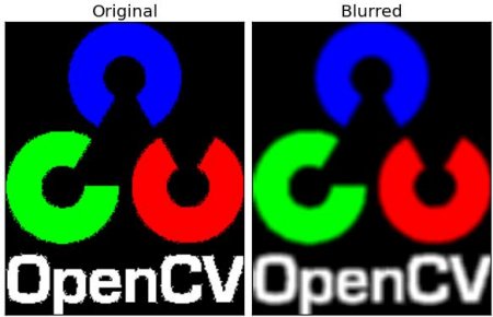
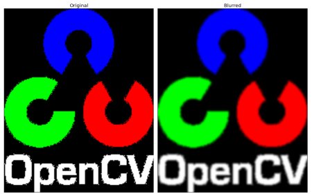
This is done by convolving an image with a normalized box filter. It simply takes the average of all the pixels under the kernel area and replaces the central element. This is done by the function cv.blur() or cv.boxFilter(). Check the docs for more details about the kernel. We should specify the width and height of the kernel. A 3×3 normalized box filter would look like the below:
Note If you don’t want to use a normalized box filter, use cv.boxFilter(). Pass an argument normalize=False to the function.
Check a sample demo below with a kernel of 5×5 size:
2. Gaussian Blurring
In this method, instead of a box filter, a Gaussian kernel is used. It is done with the function, cv.GaussianBlur(). We should specify the width and height of the kernel which should be positive and odd. We also should specify the standard deviation in the X and Y directions, sigmaX and sigmaY respectively. If only sigmaX is specified, sigmaY is taken as the same as sigmaX. If both are given as zeros, they are calculated from the kernel size. Gaussian blurring is highly effective in removing Gaussian noise from an image.
If you want, you can create a Gaussian kernel with the function, cv.getGaussianKernel().
The above code can be modified for Gaussian blurring:
3. Median Blurring
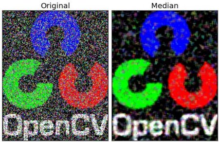
Here, the function cv.medianBlur() takes the median of all the pixels under the kernel area and the central element is replaced with this median value. This is highly effective against salt-and-pepper noise in an image. Interestingly, in the above filters, the central element is a newly calculated value which may be a pixel value in the image or a new value. But in median blurring, the central element is always replaced by some pixel value in the image. It reduces the noise effectively. Its kernel size should be a positive odd integer.
In this demo, I added a 50% noise to our original image and applied median blurring. Check the result:
4. Bilateral Filtering
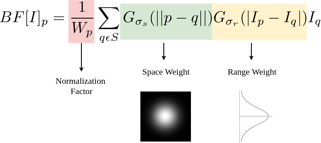
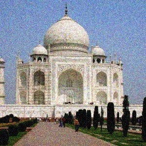
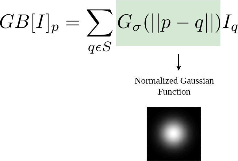
cv.bilateralFilter() is highly effective in noise removal while keeping edges sharp. But the operation is slower compared to other filters. We already saw that a Gaussian filter takes the neighbourhood around the pixel and finds its Gaussian weighted average. This Gaussian filter is a function of space alone, that is, nearby pixels are considered while filtering. It doesn’t consider whether pixels have almost the same intensity. It doesn’t consider whether a pixel is an edge pixel or not. So it blurs the edges also, which we don’t want to do.
Bilateral filtering also takes a Gaussian filter in space, but one more Gaussian filter which is a function of pixel difference. The Gaussian function of space makes sure that only nearby pixels are considered for blurring, while the Gaussian function of intensity difference makes sure that only those pixels with similar intensities to the central pixel are considered for blurring. So it preserves the edges since pixels at edges will have large intensity variation.
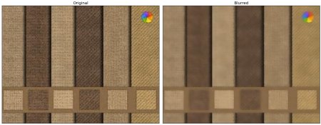
The below sample shows use of a bilateral filter (For details on arguments, visit docs).
See, the texture on the surface is gone, but the edges are still preserved.
Additional Resources
Exercises
Generated on Wed Jul 19 2023 01:37:13 for OpenCV by 1.8.13
As for one-dimensional signals, images also can be filtered with various low-pass filters (LPF), high-pass filters (HPF), etc. A LPF helps in removing noise, or blurring the image. A HPF filters helps in finding edges in an image.
OpenCV provides a function, cv2.filter2D(), to convolve a kernel with an image. As an example, we will try an averaging filter on an image. A 5×5 averaging filter kernel can be defined as follows:
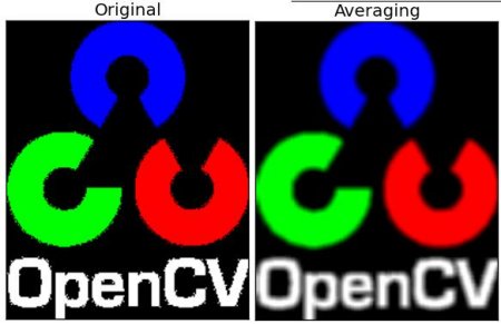


![K = \frac<1></noscript></p><p> \begin 1 & 1 & 1 & 1 & 1 \\ 1 & 1 & 1 & 1 & 1 \\ 1 & 1 & 1 & 1 & 1 \\ 1 & 1 & 1 & 1 & 1 \\ 1 & 1 & 1 & 1 & 1 \end»/></p><p>Filtering with the above kernel results in the following being performed: for each pixel, a 5×5 window is centered on this pixel, all pixels falling within this window are summed up, and the result is then divided by 25. This equates to computing the average of the pixel values inside that window. This operation is performed for all the pixels in the image to produce the output filtered image. Try this code and check the result:</p><pre><span >import</span> <span >cv2</span> <span >import</span> <span >numpy</span> <span >as</span> <span >np</span> <span >from</span> <span >matplotlib</span> <span >import</span> <span >pyplot</span> <span >as</span> <span >plt</span> <span >img</span> <span >=</span> <span >cv2</span><span >.</span><span >imread</span><span >(</span><span >'opencv_logo.png'</span><span >)</span> <span >kernel</span> <span >=</span> <span >np</span><span >.</span><span >ones</span><span >((</span><span >5</span><span >,</span><span >5</span><span >),</span><span >np</span><span >.</span><span >float32</span><span >)</span><span >/</span><span >25</span> <span >dst</span> <span >=</span> <span >cv2</span><span >.</span><span >filter2D</span><span >(</span><span >img</span><span >,</span><span >-</span><span >1</span><span >,</span><span >kernel</span><span >)</span> <span >plt</span><span >.</span><span >subplot</span><span >(</span><span >121</span><span >),</span><span >plt</span><span >.</span><span >imshow</span><span >(</span><span >img</span><span >),</span><span >plt</span><span >.</span><span >title</span><span >(</span><span >'Original'</span><span >)</span> <span >plt</span><span >.</span><span >xticks</span><span >([]),</span> <span >plt</span><span >.</span><span >yticks</span><span >([])</span> <span >plt</span><span >.</span><span >subplot</span><span >(</span><span >122</span><span >),</span><span >plt</span><span >.</span><span >imshow</span><span >(</span><span >dst</span><span >),</span><span >plt</span><span >.</span><span >title</span><span >(</span><span >'Averaging'</span><span >)</span> <span >plt</span><span >.</span><span >xticks</span><span >([]),</span> <span >plt</span><span >.</span><span >yticks</span><span >([])</span> <span >plt</span><span >.</span><span >show</span><span >()</span> </pre><p><img decoding=](https://opencv24-python-tutorials.readthedocs.io/en/latest/_images/math/220e403e44b16ea8e05d350c4ce69e9aedff5bd1.png)

![K = \frac<1></noscript></p><p> \begin 1 & 1 & 1 \\ 1 & 1 & 1 \\ 1 & 1 & 1 \end»/></p><p>If you don’t want to use a normalized box filter, use <strong>cv2.boxFilter()</strong> and pass the argument normalize=False to the function.</p><p>Check the sample demo below with a kernel of 5×5 size:</p><pre><span >import</span> <span >cv2</span> <span >import</span> <span >numpy</span> <span >as</span> <span >np</span> <span >from</span> <span >matplotlib</span> <span >import</span> <span >pyplot</span> <span >as</span> <span >plt</span> <span >img</span> <span >=</span> <span >cv2</span><span >.</span><span >imread</span><span >(</span><span >'opencv_logo.png'</span><span >)</span> <span >blur</span> <span >=</span> <span >cv2</span><span >.</span><span >blur</span><span >(</span><span >img</span><span >,(</span><span >5</span><span >,</span><span >5</span><span >))</span> <span >plt</span><span >.</span><span >subplot</span><span >(</span><span >121</span><span >),</span><span >plt</span><span >.</span><span >imshow</span><span >(</span><span >img</span><span >),</span><span >plt</span><span >.</span><span >title</span><span >(</span><span >'Original'</span><span >)</span> <span >plt</span><span >.</span><span >xticks</span><span >([]),</span> <span >plt</span><span >.</span><span >yticks</span><span >([])</span> <span >plt</span><span >.</span><span >subplot</span><span >(</span><span >122</span><span >),</span><span >plt</span><span >.</span><span >imshow</span><span >(</span><span >blur</span><span >),</span><span >plt</span><span >.</span><span >title</span><span >(</span><span >'Blurred'</span><span >)</span> <span >plt</span><span >.</span><span >xticks</span><span >([]),</span> <span >plt</span><span >.</span><span >yticks</span><span >([])</span> <span >plt</span><span >.</span><span >show</span><span >()</span> </pre><p><img decoding=](https://opencv24-python-tutorials.readthedocs.io/en/latest/_images/math/42f61cdcb41615a23af32b0fd95e674090afdc8d.png)


![GA[I]_p](https://www.geeksforgeeks.org/wp-content/ql-cache/quicklatex.com-0ab47573054042989fd4bcb26e11e4b5_l3.png)