Обучение логистической регрессии python

Logistic Regression in Machine Learning using Python

Learn how logistic regression works and how you can easily implement it from scratch using python as well as using sklearn.

In statistics logistic regression is used to model the probability of a certain class or event. I will be focusing more on the basics and implementation of the model, and not go too deep into the math part in this post.

Here the term p/(1−p) is known as the odds and denotes the likelihood of the event taking place. Thus ln(p/(1−p)) is known as the log odds and is simply used to map the probability that lies between 0 and 1 to a range between (−∞,+∞). The terms b0, b1, b2… are parameters (or weights) that we will estimate during training.

So this is just the basic math behind what we are going to do. We are interested in the probability p in this equation. So we simplify the equation to obtain the value of p:

2. Now we can easily simplify to obtain the value of p :

This actually turns out to be the equation of the Sigmoid Function which is widely used in other machine learning applications. The Sigmoid Function is given by:

Now we will be using the above derived equation to make our predictions. Before that we will train our model to obtain the values of our parameters b0, b1, b2… that result in least error. This is where the error or loss function comes in.

Loss Function

The loss is basically the error in our predicted value. In other words it is a difference between our predicted value and the actual value. We will be using the L2 Loss Function to calculate the error. Theoretically you can use any function to calculate the error. This function can be broken down as:

1. Let the actual value be yᵢ. Let the value predicted using our model be denoted as ȳᵢ. Find the difference between the actual and predicted value.
2. Square this difference.
3. Find the sum across all the values in training data.

Now that we have the error, we need to update the values of our parameters to minimize this error. This is where the “learning” actually happens, since our model is updating itself based on it’s previous output to obtain a more accurate output in the next step. Hence with each iteration our model becomes more and more accurate. We will be using the Gradient Descent Algorithm to estimate our parameters. Another commonly used algorithm is the Maximum Likelihood Estimation.

The Gradient Descent Algorithm

You might know that the partial derivative of a function at it’s minimum value is equal to 0. So gradient descent basically uses this concept to estimate the parameters or weights of our model by minimizing the loss function. Click here for a more detailed explanation on how gradient descent works.
For simplicity, for the rest of this tutorial let us assume that our output depends only on a single feature x. So we can rewrite our equation as:

Thus we need to estimate the values of weights b0 and b1 using our given training data.

1. Initially let b0=0 and b1=0. Let L be the learning rate. The learning rate controls by how much the values of b0 and b1 are updated at each step in the learning process. Here let L=0.001.
2. Calculate the partial derivative with respect to b0 and b1. The value of the partial derivative will tell us how far the loss function is from it’s minimum value. It is a measure of how much our weights need to be updated to attain minimum or ideally 0 error. In case you have more than one feature, you need to calculate the partial derivative for each weight b0, b1 … bn where n is the number of features. For a detailed explanation on the math behind calculating the partial derivatives, check out my video.

3. Next we update the values of b0 and b1:

4. We repeat this process until our loss function is a very small value or ideally reaches 0 (meaning no errors and 100% accuracy). The number of times we repeat this learning process is known as iterations or epochs.

Implementing the Model

Import the necessary libraries and download the data set here. The data was taken from kaggle and describes information about a product being purchased through an advertisement on social media. We will be predicting the value of Purchased and consider a single feature, Age to predict the values of Purchased. You can have multiple features as well.

We need to normalize our training data, and shift the mean to the origin. This is important to get accurate results because of the nature of the logistic equation. This is done by the normalize method. The predict method simply plugs in the value of the weights into the logistic model equation and returns the result. This returned value is the required probability.

The model is trained for 300 epochs or iterations. The partial derivatives are calculated at each iterations and the weights are updated. You can even calculate the loss at each step and see how it approaches zero with each step.

Implementing using Sklearn

The library sklearn can be used to perform logistic regression in a few lines as shown using the LogisticRegression class. It also supports multiple features. It requires the input values to be in a specific format hence they have been reshaped before training using the fit method.

The accuracy using this is 86.25%, which is very close to the accuracy of our model that we implemented from scratch !

Thus we have implemented a seemingly complicated algorithm easily using python from scratch and also compared it with a standard model in sklearn that does the same. I think the most crucial part here is the gradient descent algorithm, and learning how to the weights are updated at each step. Once you have learned this basic concept, then you will be able to estimate parameters for any function.

Click Here for the entire code and explanation in a Google Colaboratory. You can use it to explore and play around with the code easily.

Источник

Как выполнить логистическую регрессию в Python (шаг за шагом)

Логистическая регрессия — это метод, который мы можем использовать для подбора модели регрессии, когда переменная ответа является двоичной.

Логистическая регрессия использует метод, известный как оценка максимального правдоподобия, чтобы найти уравнение следующего вида:

log[p(X) / (1-p(X))] = β 0 + β 1 X 1 + β 2 X 2 + … + β p X p

• X j : j -я предикторная переменная
• β j : Оценка коэффициента для j -й переменной-предиктора

Формула в правой части уравнения предсказывает логарифмические шансы переменной ответа, принимающей значение 1.

Таким образом, когда мы подбираем модель логистической регрессии, мы можем использовать следующее уравнение для расчета вероятности того, что данное наблюдение примет значение 1:

p(X) = e β 0 + β 1 X 1 + β 2 X 2 + … + β p X p / (1 + e β 0 + β 1 X 1 + β 2 X 2 + … + β p X p )

Затем мы используем некоторый порог вероятности, чтобы классифицировать наблюдение как 1 или 0.

Например, мы можем сказать, что наблюдения с вероятностью больше или равной 0,5 будут классифицироваться как «1», а все остальные наблюдения будут классифицироваться как «0».

В этом руководстве представлен пошаговый пример выполнения логистической регрессии в R.

Шаг 1: Импортируйте необходимые пакеты

Во-первых, мы импортируем необходимые пакеты для выполнения логистической регрессии в Python:

import pandas as pd import numpy as np from sklearn. model_selection import train_test_split from sklearn. linear_model import LogisticRegression from sklearn import metrics import matplotlib.pyplot as plt 

Шаг 2: Загрузите данные

В этом примере мы будем использовать набор данных по умолчанию из книги Introduction to Statistical Learning.Мы можем использовать следующий код для загрузки и просмотра сводки набора данных:

#import dataset from CSV file on Github url = "https://raw.githubusercontent.com/Statology/Python-Guides/main/default.csv" data = pd.read_csv (url) #view first six rows of dataset data[0:6] default student balance income 0 0 0 729.526495 44361.625074 1 0 1 817.180407 12106.134700 2 0 0 1073.549164 31767.138947 3 0 0 529.250605 35704.493935 4 0 0 785.655883 38463.495879 5 0 1 919.588530 7491.558572 #find total observations in dataset len(data. index ) 10000 

Этот набор данных содержит следующую информацию о 10 000 человек:

• по умолчанию: указывает, нарушил ли индивидуум дефолт.
• студент: Указывает, является ли человек студентом.
• баланс: средний баланс, который несет физическое лицо.
• доход: Доход физического лица.

Мы будем использовать статус студента, банковский баланс и доход, чтобы построить модель логистической регрессии, которая предсказывает вероятность того, что данный человек не выполнит свои обязательства.

Шаг 3. Создайте обучающую и тестовую выборки

Затем мы разделим набор данных на обучающий набор для обучения модели и тестовый набор для проверки модели.

#define the predictor variables and the response variable X = data[['student', 'balance', 'income']] y = data['default'] #split the dataset into training (70%) and testing (30%) sets X_train,X_test,y_train,y_test = train_test_split (X,y,test_size=0.3,random_state=0) 

Шаг 4: Подберите модель логистической регрессии

Далее мы будем использовать функцию LogisticRegression() , чтобы подогнать модель логистической регрессии к набору данных:

#instantiate the model log_regression = LogisticRegression() #fit the model using the training data log_regression. fit (X_train,y_train) #use model to make predictions on test data y_pred = log_regression. predict (X_test) 

Шаг 5: Диагностика модели

Как только мы подойдем к регрессионной модели, мы сможем проанализировать, насколько хорошо наша модель работает с тестовым набором данных.

Во-первых, мы создадим матрицу путаницы для модели:

cnf_matrix = metrics. confusion_matrix (y_test, y_pred) cnf_matrix array([[2886, 1], [ 113, 0]]) 

Из матрицы путаницы мы видим, что:

Истинно положительных предсказаний: 2886

Истинно отрицательные прогнозы: 0

Ложноположительные прогнозы: 113

Ложноотрицательные прогнозы: 1

Мы также можем получить точность модели, которая сообщает нам процент коррекционных прогнозов, сделанных моделью:

print(" Accuracy:",metrics. accuracy_score (y_test, y_pred))l Accuracy: 0.962 

Это говорит нам о том, что модель сделала правильный прогноз относительно того, будет ли человек не выполнять свои обязательства в 96,2% случаев.

Наконец, мы можем построить кривую ROC (рабочая характеристика приемника), которая отображает процент истинных положительных результатов, предсказанных моделью, поскольку отсечка вероятности прогнозирования снижается с 1 до 0.

Чем выше AUC (площадь под кривой), тем точнее наша модель может предсказывать результаты:

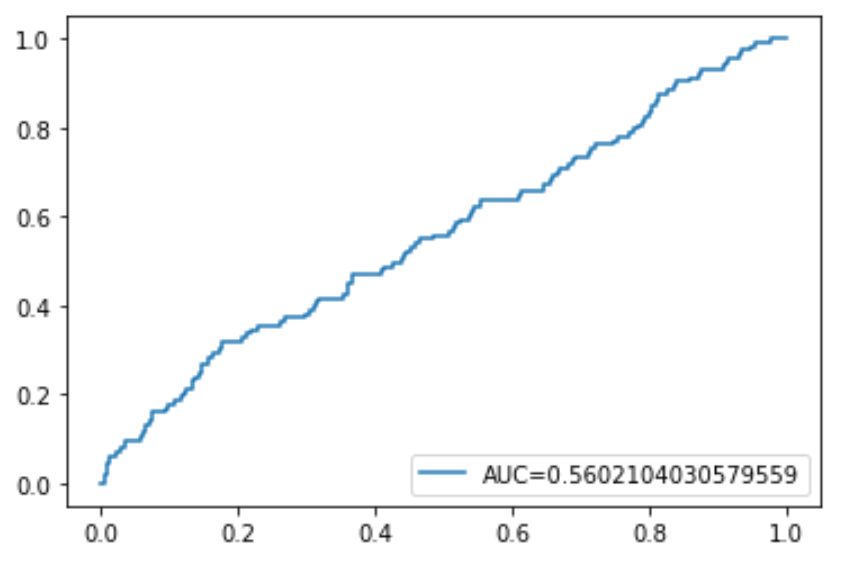
#define metrics y_pred_proba = log_regression. predict_proba (X_test)[. 1] fpr, tpr, _ = metrics. roc_curve (y_test, y_pred_proba) auc = metrics. roc_auc_score (y_test, y_pred_proba) #create ROC curve plt.plot (fpr,tpr,label=» AUC kg-card kg-image-card»>

Полный код Python, использованный в этом руководстве, можно найти здесь .

Источник