Neural networks and deep learning in python

Implementing Python in Deep Learning: An In-Depth Guide

Vihar is a developer, writer, and creator. He is currently working with the growth team at Appsmith as an Engineer and Developer Advocate.

The main idea behind deep learning is that artificial intelligence should draw inspiration from the brain. This perspective gave rise to the «neural network” terminology. The brain contains billions of neurons with tens of thousands of connections between them. Deep learning algorithms resemble the brain in many conditions, as both the brain and deep learning models involve a vast number of computation units (neurons) that are not extraordinarily intelligent in isolation but become intelligent when they interact with each other.

I think people need to understand that deep learning is making a lot of things, behind-the-scenes, much better. Deep learning is already working in Google search, and in image search; it allows you to image search a term like “hug.”— Geoffrey Hinton

Neurons

The basic building block for neural networks is artificial neurons, which imitate human brain neurons. These are simple, powerful computational units that have weighted input signals and produce an output signal using an activation function. These neurons are spread across several layers in the neural network. Below is the image of how a neuron is imitated in a neural network. The neuron takes in a input and has a particular weight with which they are connected with other neurons. Using the Activation function the nonlinearities are removed and are put into particular regions where the output is estimated. 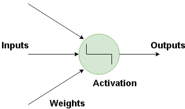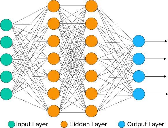Input layer : This layer consists of the neurons that do nothing than receiving the inputs and pass it on to the other layers. The number of layers in the input layer should be equal to the attributes or features in the dataset. Output Layer:The output layer is the predicted feature, it basically depends on the type of model you’re building. Hidden Layer: In between input and output layer there will be hidden layers based on the type of model. Hidden layers contain vast number of neurons. The neurons in the hidden layer apply transformations to the inputs and before passing them. As the network is trained the weights get updated, to be more predictive.

Neuron Weights

Weights refer to the strength or amplitude of a connection between two neurons, if you are familiar with linear regression you can compare weights on inputs like coefficients we use in a regression equation.Weights are often initialized to small random values, such as values in the range 0 to 1.

Feedforward Deep Networks

Feedforward supervised neural networks were among the first and most successful learning algorithms. They are also called deep networks, multi-layer Perceptron (MLP), or simply neural networks and the vanilla architecture with a single hidden layer is illustrated. Each Neuron is associated with another neuron with some weight, The network processes the input upward activating neurons as it goes to finally produce an output value. This is called a forward pass on the network. The image below depicts how data passes through the series of layers. 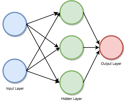There are several activation functions that are used for different use cases. The most commonly used activation functions are relu, tanh, softmax. The cheat sheet for activation functions is given below.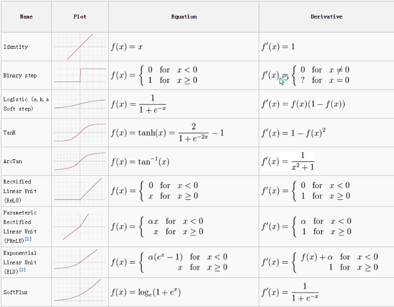

Cost Function and Gradient Descent

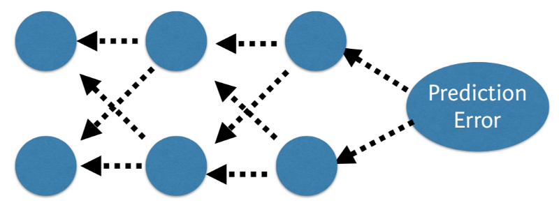
The cost function is the measure of “how good” a neural network did for its given training input and the expected output. It also may depend on attributes such as weights and biases. A cost function is single-valued, not a vector because it rates how well the neural network performed as a whole. Using the gradient descent optimization algorithm, the weights are updated incrementally after each epoch. Compatible Cost Function: Mathematically, Sum of squared errors (SSE) 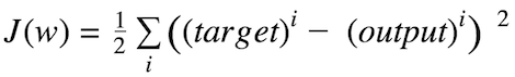The magnitude and direction of the weight update are computed by taking a step in the opposite direction of the cost gradient. 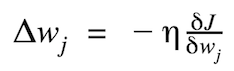where Δw is a vector that contains the weight updates of each weight coefficient w, which are computed as follows: 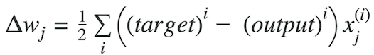Graphically, considering cost function with single coefficient We calculate the gradient descent until the derivative reaches the minimum error, and each step is determined by the steepness of the slope (gradient). 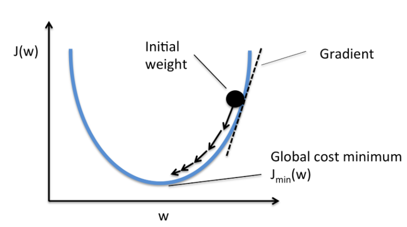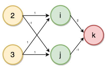Value of i will be calculated from input value and the weights corresponding to the neuron connected. i = (2 * 1) + (3 * 1) → i = 5 Similarly, j = (2 * -1) + (3 * 1) → j = 1 K = (5 * 2) + (1 * -1) → k = 9

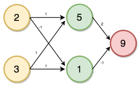
Solving the Multi Layer Perceptron problem in Python

Now that we have seen how the inputs are passed through the layers of the neural network, let’s now implement an neural network completely from scratch using a Python library called NumPy. «` # Loading the Libraries dl_multilayer_perceptron.py via GitHub

import numpy as np print("Enter the two values for input layers") print('a = ') a = int(input()) # 2 print('b = ') b = int(input()) # 3 input_data = np.array([a, b]) weights = < 'node_0': np.array([1, 1]), 'node_1': np.array([-1, 1]), 'output_node': np.array([2, -1]) >node_0_value = (input_data * weights['node_0']).sum() # 2 * 1 +3 * 1 = 5 print('node 0_hidden: <>'.format(node_0_value)) node_1_value = (input_data * weights['node_1']).sum() # 2 * -1 + 3 * 1 = 1 print('node_1_hidden: <>'.format(node_1_value)) hidden_layer_values = np.array([node_0_value, node_1_value]) output_layer = (hidden_layer_values * weights['output_node']).sum() print("output layer : <>".format(output_layer)) view raw

$python dl_multilayer_perceptron.py Enter the two values for input layers a = 3 b = 4 node 0_hidden: 7 node_1_hidden: 1 output layer : 13

Using Activation Function

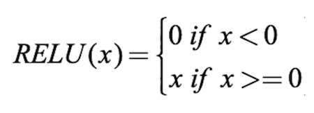
For neural Network to achieve their maximum predictive power we need to apply an activation function for the hidden layers.It is used to capture the non-linearities. We apply them to the input layers, hidden layers with some equation on the values. Here we use Rectified Linear Activation (ReLU) In the previous code snippet, we have seen how the output is generated using a simple feed-forward neural network, now in the code snippet below, we add an activation function where the sum of the product of inputs and weights are passed into the activation function. dl_fp_activation.py via GitHub

import numpy as np print("Enter the two values for input layers") print('a = ') a = int(input()) # 2 print('b = ') b = int(input()) weights = < 'node_0': np.array([2, 4]), 'node_1': np.array([[4, -5]]), 'output_node': np.array([2, 7]) >input_data = np.array([a, b]) def relu(input): # Rectified Linear Activation output = max(input, 0) return(output) node_0_input = (input_data * weights['node_0']).sum() node_0_output = relu(node_0_input) node_1_input = (input_data * weights['node_1']).sum() node_1_output = relu(node_1_input) hidden_layer_outputs = np.array([node_0_output, node_1_output]) model_output = (hidden_layer_outputs * weights['output_node']).sum() print(model_output)

$python dl_fp_activation.py Enter the two values for input layers a = 3 b = 4 44

Developing First Neural Network with Keras

About Keras: Keras is a high-level neural networks API, written in Python and capable of running on top of TensorFlow, CNTK, or Theano. It is one of the most popular frameworks for coding neural networks. Recently, Keras has been merged into tensorflow repository, boosting up more API’s and allowing multiple system usage. To install keras on your machine using PIP, run the following command.

Steps to implement your deep learning program in Keras

1. Load Data.
2. Define Model.
3. Compile Model.
4. Fit Model.
5. Evaluate Model.
6. Tie It All Together.

Developing your Keras Model

Fully connected layers are described using the Dense class. We can specify the number of neurons in the layer as the first argument, the initialisation method as the second argument as init and determine the activation function using the activation argument. Now that the model is defined, we can compile it. Compiling the model uses the efficient numerical libraries under the covers (the so-called backend) such as Theano or TensorFlow. So far we have defined our model and compiled it set for efficient computation. Now it is time to run the model on the PIMA data. We can train or fit our model on our data by calling the fit() function on the model.

Let’s get started with our program in KERAS: keras_pima.py via GitHub

# Importing Keras Sequential Model from keras.models import Sequential from keras.layers import Dense import numpy # Initializing the seed value to a integer. seed = 7 numpy.random.seed(seed) # Loading the data set (PIMA Diabetes Dataset) dataset = numpy.loadtxt('datasets/pima-indians-diabetes.csv', delimiter=",") # Loading the input values to X and Label values Y using slicing. X = dataset[:, 0:8] Y = dataset[:, 8] # Initializing the Sequential model from KERAS. model = Sequential() # Creating a 16 neuron hidden layer with Linear Rectified activation function. model.add(Dense(16, input_dim=8, init='uniform', activation='relu')) # Creating a 8 neuron hidden layer. model.add(Dense(8, init='uniform', activation='relu')) # Adding a output layer. model.add(Dense(1, init='uniform', activation='sigmoid')) # Compiling the model model.compile(loss='binary_crossentropy', optimizer='adam', metrics=['accuracy']) # Fitting the model model.fit(X, Y, nb_epoch=150, batch_size=10) scores = model.evaluate(X, Y) print("%s: %.2f%%" % (model.metrics_names[1], scores[1] * 100))

$python keras_pima.py 768/768 [==============================] - 0s - loss: 0.6776 - acc: 0.6510 Epoch 2/150 768/768 [==============================] - 0s - loss: 0.6535 - acc: 0.6510 Epoch 3/150 768/768 [==============================] - 0s - loss: 0.6378 - acc: 0.6510 . . . . . Epoch 149/150 768/768 [==============================] - 0s - loss: 0.4666 - acc: 0.7786 Epoch 150/150 768/768 [==============================] - 0s - loss: 0.4634 - acc: 0.773432/768 [>. ] - ETA: 0sacc: 77.73%

The neural network trains until 150 epochs and returns the accuracy value. The model can be used for predictions which can be achieved by the method model.

Ending Notes

Deep Learning is cutting edge technology widely used and implemented in several industries. It’s also one of the heavily researched areas in computer science. There are several neural network architectures implemented for different data types, out of these architectures, convolutional neural networks had achieved the state of the art performance in the fields of image processing techniques.

Few other architectures like Recurrent Neural Networks are applied widely for text/voice processing use cases. These neural networks, when applied to large datasets, need huge computation power and hardware acceleration, achieved by configuring Graphic Processing Units.

If you are new to using GPUs you can find free configured settings online through Kaggle Notebooks/ Google Collab Notebooks. To achieve an efficient model, one must iterate over network architecture which needs a lot of experimenting and experience. Therefore, a lot of coding practice is strongly recommended.

Источник

Deep Learning with Python: Neural Networks (complete tutorial)

Build, Plot & Explain Artificial Neural Networks with TensorFlow

Summary

In this article, I will show how to build Neural Networks with Python and how to explain Deep Learning to the Business using visualization and creating an explainer for model predictions.

Deep Learning is a type of machine learning that imitates the way humans gain certain types of knowledge, and it got more popular over the years compared to standard models. While traditional algorithms are linear, Deep Learning models, generally Neural Networks, are stacked in a hierarchy of increasing complexity and abstraction (therefore the “deep” in Deep Learning).

Neural Networks are based on a collection of connected units (neurons), which, just like the synapses in a brain, can transmit a signal to other neurons, so that, acting like interconnected brain cells, they can learn and make decisions in a more human-like manner.

Today, Deep Learning is so popular that many companies want to use it even though they don’t fully understand it. Often data scientists, first have to simplify these complex algorithms for the Business, and then explain and justify the results of the models, which is not always simple with Neural Networks. I think the best way to do it is through visualization.

I will present some useful Python code that can be easily applied in other similar cases (just copy, paste, run) and walk through every line of code with comments so that you can replicate the examples.

In particular, I will go through:

• Environment Setup, tensorflow vs pytorch.
• Artificial Neural Networks breakdown, input, output, hidden layers, activation functions.
• Deep Learning with deep neural networks.
• Model design with tensorflow/keras.
• Visualization of Neural Networks with python.
• Model training & testing.
• Explainability with shap.

Setup

There are two main libraries for building Neural Networks: TensorFlow (developed by Google) and PyTorch…

Источник