- Возникли проблемы с реализацией метода Адамса-Моултона в Python
- Saved searches
- Use saved searches to filter your results more quickly
- glider4/Adams-Bashforth-Moulton_LORENZ
- Name already in use
- Sign In Required
- Launching GitHub Desktop
- Launching GitHub Desktop
- Launching Xcode
- Launching Visual Studio Code
- Latest commit
- Git stats
- Files
- README.md
- About
- Linear Multistep methods
- Instantiation
- Adams-Bashforth Methods
- Adams-Moulton Methods
- Backward-difference formulas
- Optimal Explicit SSP methods
- Stability
- Characteristic Polynomials
- Plotting The Stability Region
Возникли проблемы с реализацией метода Адамса-Моултона в Python
Я пытаюсь реализовать метод Адамса-Моултона, используя в качестве промежуточного шага для вычисления начального числа метод Ньютона-Рафсона. Получил следующее:
from pylab import * from time import perf_counter def AM3c(a,b,N,y0,fun,dfun): y = zeros(N+1) yy = zeros(N+1) t = zeros(N+1) f = zeros(N+1) C = zeros(N+1) L = zeros(N+1) t[0] = a h = (b-a)/float(N) y[0] = y0 yy[0] = y0 f[0] = fun(a,y[0]) y[1] = y[0] + h*f[0] t[1] = a+h f[1] = fun(t[1], y[1]) t[2] = t[1]+h K1 = fun(t[1],y[1]) K2 = fun(t[1]+h/2,y[1]+h/2*K1) K3 = fun(t[1]+h/2,y[1]+h/2*K2) K4 = fun(t[1]+h,y[1]+h*K3) y[2] = y[1]+h/6*(K1+2*K2+2*K3+K4) f[2] = fun(t[2],y[2]) for k in range(2,N): C[k] = y[k] + h/24*(19*f[k] - 5*f[k-1] + f[k-2]) t[k+1] = t[k] + h z = zeros(201) z[0] = y[k] error = 1. l = 0 while (error > 1.e-12) and (l<200): z[l+1] = z[l]-(fun(t[k+1],z[l]))/(dfun(t[k+1],z[l])) error = abs(z[l+1]-z[l]) yy[k+1] = z[l+1] l +=1 L[k+1] = l y[k+1] = h*9/24*fun(t[k+1],yy[k+1])+ C[k] f[k+1] = fun(t[k+1], y[k+1]) return (t,y,L) Насколько я знаю, это кажется правильным. Но когда я рисую приближения функции ниже для разных N, результаты не очень хороши:
def fun(t,y): return -y+exp(-t)*cos(t); def exact(t): return exp(-t)*sin(t); def dfun(t,y): return -1; y0 = 0.0 a = 0.0 b = 5.0 set = [10,20,40,80,160] figure('AM3 Newton') for N in set: tini = perf_counter() (t,y,L) = AM3c(a,b,N,y0,fun,df) tfin = perf_counter() ye = exact(t) plot(t,y, '*-') h = (b - a)/float(N) error = max(abs(y-ye)) tcpu = tfin-tini maxiter = max(L) print('---------------') print('h: '+ str(h)) print('Error: '+str(error)) print('Time CPU: '+str(tcpu)) if (maxiter == 200): print('The algorithm doesn't converge, therefore the method doesn't work properly') else: print('Max no. of iterations: ' + str(maxiter-1)) plot(t,ye,'k') legend(['N=10','N=20','N=40','N=80','N=160','Exact']) Это также показывает ошибку программы, количество итераций, выполняемых методом Ньютона-Рафсона, и время, необходимое ЦП для создания программы.
При реализации этого с другой функцией программа дает очень плохие приближения. Например, с этой функцией:
def f(t,y): return 1 + y**2; def df(t,y): return 2*y; def exact(t): return tan(t); a = 0 b = 1 y0 = 0 N = 320 tini = perf_counter() (t,y,L) = AM3c(a,b,N,y0,f,df) tfin = perf_counter() ye = exact(t) plot(t,y, '*-') h = (b - a)/float(N) tcpu = tfin-tini maxiter = max(L) print('---------------') print('h: '+ str(h)) print('Time CPU: '+str(tcpu)) if (maxiter == 200): print('The algorithm doesn't converge, therefore the method doesn't work properly') else: print('Max no. of iterations: ' + str(maxiter-1)) plot(t,ye,'k') legend(['N=320','Exact']) Для контекста я получил "нормальный" метод Адамса-Моултона следующим образом:
def AM3b(a,b,N,y0,fun,dfun): y = zeros(N+1) yy = zeros(N+1) t = zeros(N+1) f = zeros(N+1) C = zeros(N+1) L = zeros(N+1) t[0] = a h = (b-a)/float(N) y[0] = y0 yy[0] = y0 f[0] = fun(a,y[0]) y[1] = y[0] + h*f[0] t[1] = a+h f[1] = fun(t[1], y[1]) t[2] = t[1]+h K1 = fun(t[1],y[1]) K2 = fun(t[1]+h/2,y[1]+h/2*K1) K3 = fun(t[1]+h/2,y[1]+h/2*K2) K4 = fun(t[1]+h,y[1]+h*K3) y[2] = y[1]+h/6*(K1+2*K2+2*K3+K4) f[2] = fun(t[2],y[2]) for k in range(2,N): C[k] = y[k] + h/24*(19*f[k] - 5*f[k-1] + f[k-2]) t[k+1] = t[k] + h z = zeros(201) z[0] = y[k] error = 1. l = 0 while (error > 1.e-12) and (l<200): z[l+1] = h*9./24*fun(t[k+1],z[l])+C[k] error = abs(z[l+1]-z[l]) yy[k+1] = z[l+1] l +=1 L[k+1] = l y[k+1] = h*9/24*fun(t[k+1],yy[k+1])+ C[k] f[k+1] = fun(t[k+1], y[k+1]) return (t,y,L) который отлично работает (единственная разница - семя z[k+1] ).
Разве я не реализовал метод NR в методе AM? Или такие результаты должны иметь место?
Заранее спасибо! И, кстати, я использую Python 3.8.5 на тот случай, если у кого-то есть более низкая версия и возникнут проблемы с ее запуском.
Saved searches
Use saved searches to filter your results more quickly
You signed in with another tab or window. Reload to refresh your session. You signed out in another tab or window. Reload to refresh your session. You switched accounts on another tab or window. Reload to refresh your session.
Using the Adams-Bashforth-Moulton method (with Runge-Kutta 4th order) to approximate the Lorenz problem. 3D result plotting using matplotlib.
glider4/Adams-Bashforth-Moulton_LORENZ
This commit does not belong to any branch on this repository, and may belong to a fork outside of the repository.
Name already in use
A tag already exists with the provided branch name. Many Git commands accept both tag and branch names, so creating this branch may cause unexpected behavior. Are you sure you want to create this branch?
Sign In Required
Please sign in to use Codespaces.
Launching GitHub Desktop
If nothing happens, download GitHub Desktop and try again.
Launching GitHub Desktop
If nothing happens, download GitHub Desktop and try again.
Launching Xcode
If nothing happens, download Xcode and try again.
Launching Visual Studio Code
Your codespace will open once ready.
There was a problem preparing your codespace, please try again.
Latest commit
Git stats
Files
Failed to load latest commit information.
README.md
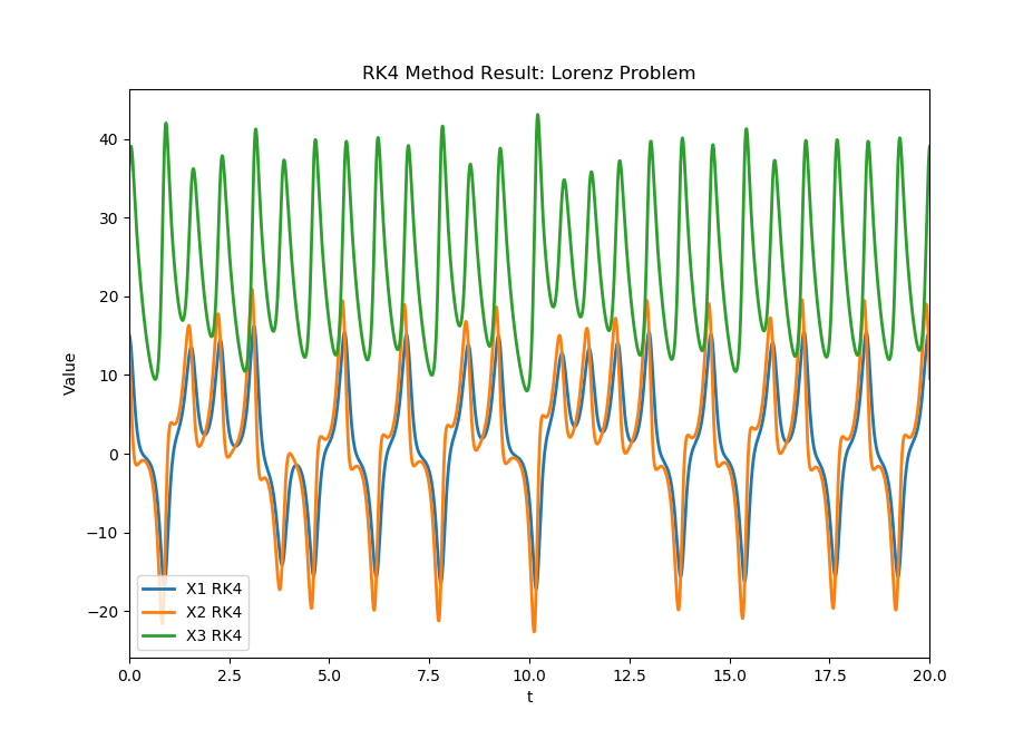
Using the Adams-Bashforth-Moulton method (via Runge-Kutta 4th order) to approximate the Lorenz problem. Firstly starting with RK4 alone to see how the accuracy compares before implementing ABM. ABM then uses RK4 as part of its computation. I ran ABM up to n=1,000,000.
RK 4 Solo Solution: n=100,000

Adams-Bashforth-Moulton Solution, n=1,000,000

About
Using the Adams-Bashforth-Moulton method (with Runge-Kutta 4th order) to approximate the Lorenz problem. 3D result plotting using matplotlib.
Linear Multistep methods
A linear multistep method computes the next solution value from the values at several previous steps:
$$ \alpha_k y_ + \alpha_ y_ + \cdots + \alpha_0 y_n = h ( \beta_k f_ + \cdots + \beta_0 f_n ) $$
Note that different conventions for numbering the coefficients exist; the above form is used in NodePy. Methods are automatically normalized so that \(\alpha_k=1\) .
>>> import nodepy.linear_multistep_method as lm >>> ab3=lm.Adams_Bashforth(3) >>> ab3.order() 3 >>> bdf2=lm.backward_difference_formula(2) >>> bdf2.order() 2 >>> bdf2.is_zero_stable() True >>> bdf7=lm.backward_difference_formula(7) >>> bdf7.is_zero_stable() False >>> bdf3=lm.backward_difference_formula(3) >>> bdf3.A_alpha_stability() 86 >>> ssp32=lm.elm_ssp2(3) >>> ssp32.order() 2 >>> ssp32.ssp_coefficient() 1/2 >>> ssp32.plot_stability_region()
Instantiation
The follwing functions return linear multistep methods of some common types:
- Adams-Bashforth methods: Adams_Bashforth(k)
- Adams-Moulton methods: Adams_Moulton(k)
- backward_difference_formula(k)
- Optimal explicit SSP methods (elm_ssp2(k))
In each case, the argument \(k\) specifies the number of steps in the method. Note that it is possible to generate methods for arbitrary \(k\) , but currently for large \(k\) there are large errors in the coefficients due to roundoff errors. This begins to be significant at 7 steps. However, members of these families with many steps do not have good properties.
More generally, a linear multistep method can be instantiated by specifying its coefficients \(\alpha, \beta\) :
>> from nodepy import linear_multistep_method as lmm >> my_lmm=lmm.LinearMultistepMethod(alpha,beta)
Adams-Bashforth Methods
Construct the k-step, Adams-Bashforth method. The methods are explicit and have order k. They have the form:
They are generated using equations (1.5) and (1.7) from [HNorW93] III.1, along with the binomial expansion.
>>> import nodepy.linear_multistep_method as lm >>> ab3=lm.Adams_Bashforth(3) >>> print(ab3) 3-step Adams-Bashforth Explicit 3-step method of order 3 alpha = [ 0 0 -1 1 ] beta = [ 5/12 -4/3 23/12 0 ] >>> ab3.order() 3
Adams-Moulton Methods
Construct the \(k\) -step, Adams-Moulton method. The methods are implicit and have order \(k+1\) . They have the form:
They are generated using equation (1.9) and the equation in Exercise 3 from Hairer & Wanner III.1, along with the binomial expansion.
>>> import nodepy.linear_multistep_method as lm >>> am3=lm.Adams_Moulton(3) >>> am3.order() 4
Backward-difference formulas
Construct the \(k\) -step backward differentiation method. The methods are implicit and have order \(k\) .
They are generated using equation (1.22’) from Hairer & Wanner III.1, along with the binomial expansion.
>>> import nodepy.linear_multistep_method as lm >>> bdf4=lm.backward_difference_formula(4) >>> bdf4.A_alpha_stability() 73
Reference: [HNorW93] pp. 364-365
Optimal Explicit SSP methods
Returns the optimal SSP \(k\) -step linear multistep method of order 2.
>>> import nodepy.linear_multistep_method as lm >>> lm10=lm.elm_ssp2(10) >>> lm10.ssp_coefficient() 8/9
Stability
Characteristic Polynomials
Returns the characteristic polynomials (also known as generating polynomials) of a linear multistep method. They are:
>>> from nodepy import lm >>> ab5 = lm.Adams_Bashforth(5) >>> rho,sigma = ab5.characteristic_polynomials() >>> print(rho) 5 4 1 x - 1 x >>> print(sigma) 4 3 2 2.64 x - 3.853 x + 3.633 x - 1.769 x + 0.3486
Reference: [HNorW93] p. 370, eq. 2.4
Plotting The Stability Region
LinearMultistepMethod. plot_stability_region ( N = 100 , bounds = None , color = 'r' , filled = True , alpha = 1.0 , to_file = False , longtitle = False ) [source]
The region of absolute stability of a linear multistep method is the set
where \(\rho(\zeta)\) and \(\sigma(\zeta)\) are the characteristic functions of the method.
Also plots the boundary locus, which is given by the set of points z:
Here \(\rho\) and \(\sigma\) are the characteristic polynomials of the method.
Reference: [LeV07] section 7.6.1
- N – Number of gridpoints to use in each direction
- bounds – limits of plotting region
- color – color to use for this plot
- filled – if true, stability region is filled in (solid); otherwise it is outlined