Matplotlib python цвет линии

Specifying colors#

Matplotlib recognizes the following formats to specify a color.

RGB or RGBA (red, green, blue, alpha) tuple of float values in a closed interval [0, 1].

Case-insensitive hex RGB or RGBA string.

Case-insensitive RGB or RGBA string equivalent hex shorthand of duplicated characters.

String representation of float value in closed interval [0, 1] for grayscale values.

Single character shorthand notation for some basic colors.

The colors green, cyan, magenta, and yellow do not coincide with X11/CSS4 colors. Their particular shades were chosen for better visibility of colored lines against typical backgrounds.

• ‘b’ as blue
• ‘g’ as green
• ‘r’ as red
• ‘c’ as cyan
• ‘m’ as magenta
• ‘y’ as yellow
• ‘k’ as black
• ‘w’ as white

Case-insensitive X11/CSS4 color name with no spaces.

Case-insensitive color name from xkcd color survey with ‘xkcd:’ prefix.

Case-insensitive Tableau Colors from ‘T10’ categorical palette.

This is the default color cycle.

• ‘tab:blue’
• ‘tab:orange’
• ‘tab:green’
• ‘tab:red’
• ‘tab:purple’
• ‘tab:brown’
• ‘tab:pink’
• ‘tab:gray’
• ‘tab:olive’
• ‘tab:cyan’

«CN» color spec where ‘C’ precedes a number acting as an index into the default property cycle.

Matplotlib indexes color at draw time and defaults to black if cycle does not include color.

rcParams[«axes.prop_cycle»] (default: cycler(‘color’, [‘#1f77b4’, ‘#ff7f0e’, ‘#2ca02c’, ‘#d62728’, ‘#9467bd’, ‘#8c564b’, ‘#e377c2’, ‘#7f7f7f’, ‘#bcbd22’, ‘#17becf’]) )

«Red», «Green», and «Blue» are the intensities of those colors. In combination, they represent the colorspace.

Transparency#

The alpha value of a color specifies its transparency, where 0 is fully transparent and 1 is fully opaque. When a color is semi-transparent, the background color will show through.

The alpha value determines the resulting color by blending the foreground color with the background color according to the formula

The following plot illustrates the effect of transparency.

import matplotlib.pyplot as plt from matplotlib.patches import Rectangle import numpy as np fig, ax = plt.subplots(figsize=(6.5, 1.65), layout='constrained') ax.add_patch(Rectangle((-0.2, -0.35), 11.2, 0.7, color='C1', alpha=0.8)) for i, alpha in enumerate(np.linspace(0, 1, 11)): ax.add_patch(Rectangle((i, 0.05), 0.8, 0.6, alpha=alpha, zorder=0)) ax.text(i+0.4, 0.85, f"alpha:.1f>", ha='center') ax.add_patch(Rectangle((i, -0.05), 0.8, -0.6, alpha=alpha, zorder=2)) ax.set_xlim(-0.2, 13) ax.set_ylim(-1, 1) ax.set_title('alpha values') ax.text(11.3, 0.6, 'zorder=1', va='center', color='C0') ax.text(11.3, 0, 'zorder=2\nalpha=0.8', va='center', color='C1') ax.text(11.3, -0.6, 'zorder=3', va='center', color='C0') ax.axis('off') 

The orange rectangle is semi-transparent with alpha = 0.8. The top row of blue squares is drawn below and the bottom row of blue squares is drawn on top of the orange rectangle.

See also Zorder Demo to learn more on the drawing order.

«CN» color selection#

Matplotlib converts «CN» colors to RGBA when drawing Artists. The Styling with cycler section contains additional information about controlling colors and style properties.

import numpy as np import matplotlib.pyplot as plt import matplotlib as mpl th = np.linspace(0, 2*np.pi, 128) def demo(sty): mpl.style.use(sty) fig, ax = plt.subplots(figsize=(3, 3)) ax.set_title('style: '.format(sty), color='C0') ax.plot(th, np.cos(th), 'C1', label='C1') ax.plot(th, np.sin(th), 'C2', label='C2') ax.legend() demo('default') demo('seaborn-v0_8') 

• 
• 

The first color ‘C0’ is the title. Each plot uses the second and third colors of each style’s rcParams[«axes.prop_cycle»] (default: cycler(‘color’, [‘#1f77b4’, ‘#ff7f0e’, ‘#2ca02c’, ‘#d62728’, ‘#9467bd’, ‘#8c564b’, ‘#e377c2’, ‘#7f7f7f’, ‘#bcbd22’, ‘#17becf’]) ). They are ‘C1’ and ‘C2’ , respectively.

Comparison between X11/CSS4 and xkcd colors#

95 out of the 148 X11/CSS4 color names also appear in the xkcd color survey. Almost all of them map to different color values in the X11/CSS4 and in the xkcd palette. Only ‘black’, ‘white’ and ‘cyan’ are identical.

For example, ‘blue’ maps to ‘#0000FF’ whereas ‘xkcd:blue’ maps to ‘#0343DF’ . Due to these name collisions, all xkcd colors have the ‘xkcd:’ prefix.

The visual below shows name collisions. Color names where color values agree are in bold.

import matplotlib.colors as mcolors import matplotlib.patches as mpatch overlap = name for name in mcolors.CSS4_COLORS if f'xkcd:name>' in mcolors.XKCD_COLORS> fig = plt.figure(figsize=[9, 5]) ax = fig.add_axes([0, 0, 1, 1]) n_groups = 3 n_rows = len(overlap) // n_groups + 1 for j, color_name in enumerate(sorted(overlap)): css4 = mcolors.CSS4_COLORS[color_name] xkcd = mcolors.XKCD_COLORS[f'xkcd:color_name>'].upper() # Pick text colour based on perceived luminance. rgba = mcolors.to_rgba_array([css4, xkcd]) luma = 0.299 * rgba[:, 0] + 0.587 * rgba[:, 1] + 0.114 * rgba[:, 2] css4_text_color = 'k' if luma[0] > 0.5 else 'w' xkcd_text_color = 'k' if luma[1] > 0.5 else 'w' col_shift = (j // n_rows) * 3 y_pos = j % n_rows text_args = dict(fontsize=10, weight='bold' if css4 == xkcd else None) ax.add_patch(mpatch.Rectangle((0 + col_shift, y_pos), 1, 1, color=css4)) ax.add_patch(mpatch.Rectangle((1 + col_shift, y_pos), 1, 1, color=xkcd)) ax.text(0.5 + col_shift, y_pos + .7, css4, color=css4_text_color, ha='center', **text_args) ax.text(1.5 + col_shift, y_pos + .7, xkcd, color=xkcd_text_color, ha='center', **text_args) ax.text(2 + col_shift, y_pos + .7, f' color_name>', **text_args) for g in range(n_groups): ax.hlines(range(n_rows), 3*g, 3*g + 2.8, color='0.7', linewidth=1) ax.text(0.5 + 3*g, -0.3, 'X11/CSS4', ha='center') ax.text(1.5 + 3*g, -0.3, 'xkcd', ha='center') ax.set_xlim(0, 3 * n_groups) ax.set_ylim(n_rows, -1) ax.axis('off') plt.show() 

Total running time of the script: ( 0 minutes 2.179 seconds)

Источник

Использование библиотеки Matplotlib. Как менять стиль линий на одномерном графике

В предыдущем примере мы рисовали простейшие графики, а теперь научимся изменять стиль линий, которыми они рисуются.

Есть несколько способов описания стиля линий.

Задание стиля в виде строки

Первый и самый простой способ состоит в использовании дополнительного третьего текстового параметра функции plot() из пакета pyplot. Строка стиля может включать в себя три компонента: цвет линии, стиль линии, маркер. В следующих двух таблицах таблице показаны символы, обозначающие стили и маркеры.

Символ стиля	Результат
—
—
-.
:
.
,

Символ маркера	Результат
o
v
^
>
1
2
3
4
s
p
*
h
H
+
x
D
d
|
_

Например, если нужно нарисовать график штриховой линией, то в качестве стиля нужно указать «—«. Для отображения графика сплошной линией с маркером в виде кружочков можно использовать стиль «-o». Если же мы хотим сделать цвет графика, например, красным, то можно добавить букву, отвечающую за красный цвет («r»): «-or».

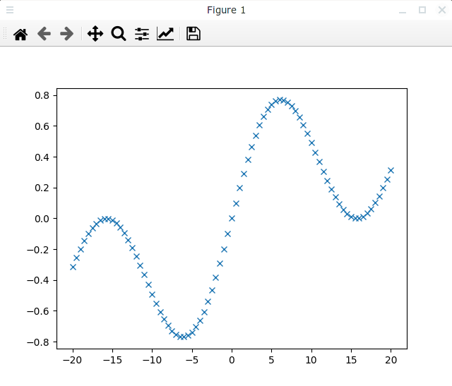
Следующий пример рисует график функции с использованием стиля «x», когда график представляет собой последовательность крестиков, не соединенных между собой линиями. Поскольку цвет не указан, то используется цвет по умолчанию.

# . Импортируем один из пакетов Matplotlib
import matplotlib. pyplot as plt

if __name__ == ‘__main__’ :
# Интервал изменения переменной по оси X
xmin = — 20.0
xmax = 20.0

# . Создадим список координат по оси X на отрезке [xmin; xmax], включая концы
x = np. arange ( xmin , xmax + dx , dx )

# Вычислим функцию на заданном интервале
y = np. sin ( 0.2 * x ) * np. cos ( 0.1 * x )

# . Нарисуем одномерный график с использованием стиля
plt. plot ( x , y , «x» )

# . Покажем окно с нарисованным графиком
plt. show ( )

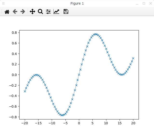
Давайте скомбинируем стиль линии и метки. Например, если в предыдущем примере заменить вызов функции plot() на следующую:

то мы получим следующий график:

Два стиля маркера указывать нельзя, в этом случае мы получим ошибку.

Кроме обозначения стиля в строке может содержаться символ, описывающий цвет графика, но здесь мы ограничены следующими цветами:

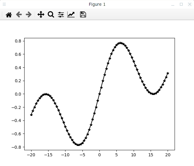
Например, следующая строка кода рисует график черной линией, на которой которую наносятся маркеры в виде звездочек

Более гибкий способ задания стиля

Другой способ более гибкий, в том числе в плане задания цветов. Он состоит в том, чтобы в явном виде задавать различные параметры линии. В этом случае один параметр, который отвечал за стиль в прошлых примерах, разобьем на несколько параметров:

Кроме того, можно использовать дополнительные параметры. Например:

• markerfacecolor — цвет маркеров.
• markersize — размер маркера.
• linewidth или lw — толщина линии.

Есть еще и другие параметры, но о них мы пока говорить не будем.

Если в первом способе мы были ограничены восемью цветами, то теперь цвета настраиваются более гибко. О том, как можно задавать цвета я уже писал в статье Способы задания цвета в Matplotlib.

Источник

matplotlib.pyplot.plot#

The coordinates of the points or line nodes are given by x, y.

The optional parameter fmt is a convenient way for defining basic formatting like color, marker and linestyle. It’s a shortcut string notation described in the Notes section below.

>>> plot(x, y) # plot x and y using default line style and color >>> plot(x, y, 'bo') # plot x and y using blue circle markers >>> plot(y) # plot y using x as index array 0..N-1 >>> plot(y, 'r+') # ditto, but with red plusses 

You can use Line2D properties as keyword arguments for more control on the appearance. Line properties and fmt can be mixed. The following two calls yield identical results:

>>> plot(x, y, 'go--', linewidth=2, markersize=12) >>> plot(x, y, color='green', marker='o', linestyle='dashed', . linewidth=2, markersize=12) 

When conflicting with fmt, keyword arguments take precedence.

Plotting labelled data

There’s a convenient way for plotting objects with labelled data (i.e. data that can be accessed by index obj[‘y’] ). Instead of giving the data in x and y, you can provide the object in the data parameter and just give the labels for x and y:

>>> plot('xlabel', 'ylabel', data=obj) 

All indexable objects are supported. This could e.g. be a dict , a pandas.DataFrame or a structured numpy array.

Plotting multiple sets of data

There are various ways to plot multiple sets of data.

The most straight forward way is just to call plot multiple times. Example:

>>> plot(x1, y1, 'bo') >>> plot(x2, y2, 'go') 

>>> x = [1, 2, 3] >>> y = np.array([[1, 2], [3, 4], [5, 6]]) >>> plot(x, y) 

>>> for col in range(y.shape[1]): . plot(x, y[:, col]) 

By default, each line is assigned a different style specified by a ‘style cycle’. The fmt and line property parameters are only necessary if you want explicit deviations from these defaults. Alternatively, you can also change the style cycle using rcParams[«axes.prop_cycle»] (default: cycler(‘color’, [‘#1f77b4’, ‘#ff7f0e’, ‘#2ca02c’, ‘#d62728’, ‘#9467bd’, ‘#8c564b’, ‘#e377c2’, ‘#7f7f7f’, ‘#bcbd22’, ‘#17becf’]) ).

Parameters : x, y array-like or scalar

The horizontal / vertical coordinates of the data points. x values are optional and default to range(len(y)) .

Commonly, these parameters are 1D arrays.

They can also be scalars, or two-dimensional (in that case, the columns represent separate data sets).

These arguments cannot be passed as keywords.

fmt str, optional

A format string, e.g. ‘ro’ for red circles. See the Notes section for a full description of the format strings.

Format strings are just an abbreviation for quickly setting basic line properties. All of these and more can also be controlled by keyword arguments.

This argument cannot be passed as keyword.

data indexable object, optional

An object with labelled data. If given, provide the label names to plot in x and y.

Technically there’s a slight ambiguity in calls where the second label is a valid fmt. plot(‘n’, ‘o’, data=obj) could be plt(x, y) or plt(y, fmt) . In such cases, the former interpretation is chosen, but a warning is issued. You may suppress the warning by adding an empty format string plot(‘n’, ‘o’, », data=obj) .

A list of lines representing the plotted data.

Other Parameters : scalex, scaley bool, default: True

These parameters determine if the view limits are adapted to the data limits. The values are passed on to autoscale_view .

**kwargs Line2D properties, optional

kwargs are used to specify properties like a line label (for auto legends), linewidth, antialiasing, marker face color. Example:

>>> plot([1, 2, 3], [1, 2, 3], 'go-', label='line 1', linewidth=2) >>> plot([1, 2, 3], [1, 4, 9], 'rs', label='line 2') 

If you specify multiple lines with one plot call, the kwargs apply to all those lines. In case the label object is iterable, each element is used as labels for each set of data.

Here is a list of available Line2D properties:

a filter function, which takes a (m, n, 3) float array and a dpi value, and returns a (m, n, 3) array and two offsets from the bottom left corner of the image

Источник