- matplotlib.pyplot.scatter#
- Matplotlib. Урок 4.2. Визуализация данных. Ступенчатый, стековый, точечный график и другие
- Ступенчатый график
- Стековый график
- Stem-график
- Точечный график
- Статьи с описанием различных вариантов работы с точечными графиками
- P.S.
- Matplotlib. Урок 4.2. Визуализация данных. Ступенчатый, стековый, точечный график и другие : 1 комментарий
- Plot types#
- Basic#
- Plots of arrays and fields#
- Statistics plots#
- Unstructured coordinates#
- 3D#
matplotlib.pyplot.scatter#
matplotlib.pyplot. scatter ( x , y , s = None , c = None , marker = None , cmap = None , norm = None , vmin = None , vmax = None , alpha = None , linewidths = None , * , edgecolors = None , plotnonfinite = False , data = None , ** kwargs ) [source] #
A scatter plot of y vs. x with varying marker size and/or color.
Parameters : x, y float or array-like, shape (n, )
s float or array-like, shape (n, ), optional
The marker size in points**2 (typographic points are 1/72 in.). Default is rcParams[‘lines.markersize’] ** 2 .
c array-like or list of colors or color, optional
The marker colors. Possible values:
- A scalar or sequence of n numbers to be mapped to colors using cmap and norm.
- A 2D array in which the rows are RGB or RGBA.
- A sequence of colors of length n.
- A single color format string.
Note that c should not be a single numeric RGB or RGBA sequence because that is indistinguishable from an array of values to be colormapped. If you want to specify the same RGB or RGBA value for all points, use a 2D array with a single row. Otherwise, value-matching will have precedence in case of a size matching with x and y.
If you wish to specify a single color for all points prefer the color keyword argument.
Defaults to None . In that case the marker color is determined by the value of color, facecolor or facecolors. In case those are not specified or None , the marker color is determined by the next color of the Axes ‘ current «shape and fill» color cycle. This cycle defaults to rcParams[«axes.prop_cycle»] (default: cycler(‘color’, [‘#1f77b4’, ‘#ff7f0e’, ‘#2ca02c’, ‘#d62728’, ‘#9467bd’, ‘#8c564b’, ‘#e377c2’, ‘#7f7f7f’, ‘#bcbd22’, ‘#17becf’]) ).
The marker style. marker can be either an instance of the class or the text shorthand for a particular marker. See matplotlib.markers for more information about marker styles.
cmap str or Colormap , default: rcParams[«image.cmap»] (default: ‘viridis’ )
The Colormap instance or registered colormap name used to map scalar data to colors.
This parameter is ignored if c is RGB(A).
norm str or Normalize , optional
The normalization method used to scale scalar data to the [0, 1] range before mapping to colors using cmap. By default, a linear scaling is used, mapping the lowest value to 0 and the highest to 1.
If given, this can be one of the following:
- An instance of Normalize or one of its subclasses (see Colormap Normalization ).
- A scale name, i.e. one of «linear», «log», «symlog», «logit», etc. For a list of available scales, call matplotlib.scale.get_scale_names() . In that case, a suitable Normalize subclass is dynamically generated and instantiated.
This parameter is ignored if c is RGB(A).
vmin, vmax float, optional
When using scalar data and no explicit norm, vmin and vmax define the data range that the colormap covers. By default, the colormap covers the complete value range of the supplied data. It is an error to use vmin/vmax when a norm instance is given (but using a str norm name together with vmin/vmax is acceptable).
This parameter is ignored if c is RGB(A).
alpha float, default: None
The alpha blending value, between 0 (transparent) and 1 (opaque).
linewidths float or array-like, default: rcParams[«lines.linewidth»] (default: 1.5 )
The linewidth of the marker edges. Note: The default edgecolors is ‘face’. You may want to change this as well.
edgecolors None> or color or sequence of color, default: rcParams[«scatter.edgecolors»] (default: ‘face’ )
The edge color of the marker. Possible values:
- ‘face’: The edge color will always be the same as the face color.
- ‘none’: No patch boundary will be drawn.
- A color or sequence of colors.
For non-filled markers, edgecolors is ignored. Instead, the color is determined like with ‘face’, i.e. from c, colors, or facecolors.
plotnonfinite bool, default: False
Whether to plot points with nonfinite c (i.e. inf , -inf or nan ). If True the points are drawn with the bad colormap color (see Colormap.set_bad ).
Returns : PathCollection Other Parameters : data indexable object, optional
If given, the following parameters also accept a string s , which is interpreted as data[s] (unless this raises an exception):
**kwargs Collection properties
To plot scatter plots when markers are identical in size and color.
- The plot function will be faster for scatterplots where markers don’t vary in size or color.
- Any or all of x, y, s, and c may be masked arrays, in which case all masks will be combined and only unmasked points will be plotted.
- Fundamentally, scatter works with 1D arrays; x, y, s, and c may be input as N-D arrays, but within scatter they will be flattened. The exception is c, which will be flattened only if its size matches the size of x and y.
Matplotlib. Урок 4.2. Визуализация данных. Ступенчатый, стековый, точечный график и другие


В этому уроке рассмотрим на примерах работу со ступенчатым, стековым, stem-графиком и точечным графиком.
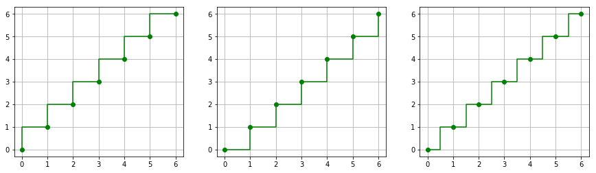
Ступенчатый график
Рассмотрим еще одни график – ступенчатый. Такой график строится с помощью функции step() , которая принимает следующий набор параметров:
- x: array_like
- набор данных для оси абсцисс
- набор данных для оси ординат
- Задает отображение линии (см. функцию plot() ).
- метки
- Определяет место, где будет установлен шаг.
- ‘pre’ : значение y ставится слева от значения x , т.е. значение y[i] определяется для интервала (x[i-1]; x[i]) .
- ‘post’ : значение y ставится справа от значения x , т.е. значение y[i] определяется для интервала (x[i]; x[i+1]) .
- ‘mid’ : значение y ставится в середине интервала.
x = np.arange(0, 7) y = x where_set = ['pre', 'post', 'mid'] fig, axs = plt.subplots(1, 3, figsize=(15, 4)) for i, ax in enumerate(axs): ax.step(x, y, "g-o", where=where_set[i]) ax.grid()

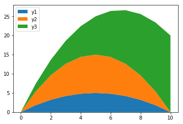
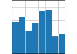
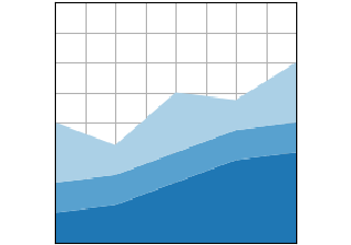
Стековый график
Для построения стекового графика используется функция stackplot() . Суть его в том, что графики отображаются друг над другом, и каждый следующий является суммой предыдущего и заданного набора данных:
x = np.arange(0, 11, 1) y1 = np.array([(-0.2)*i**2+2*i for i in x]) y2 = np.array([(-0.4)*i**2+4*i for i in x]) y3 = np.array([2*i for i in x]) labels = ["y1", "y2", "y3"] fig, ax = plt.subplots() ax.stackplot(x, y1, y2, y3, labels=labels) ax.legend(loc='upper left')
Верхний край области y2 определяется как сумма значений из наборов y1 и y2 , y3 – соответственно сумма y1 , y2 и y3 .
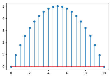
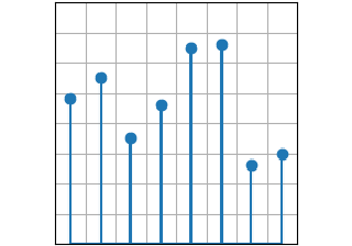
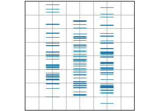
Stem-график
Визуально этот график выглядит как набор линий от точки с координатами ( x , y ) до базовой линии, в верхней точке ставится маркер:
x = np.arange(0, 10.5, 0.5) y = np.array([(-0.2)*i**2+2*i for i in x]) plt.stem(x, y)
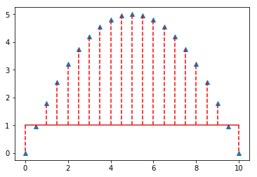
Дополнительные параметры функции stem() :
Реализуем пример, демонстрирующий работу с дополнительными параметрами:
plt.stem(x, y, linefmt="r--", markerfmt="^", bottom=1)
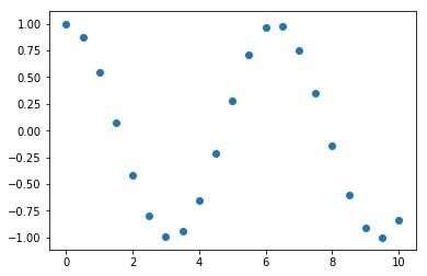
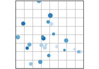
Точечный график
Для отображения точечного графика предназначена функция scatter() . В простейшем виде точечный график можно получить передав функции scatter() наборы точек для x , y координат:
x = np.arange(0, 10.5, 0.5) y = np.cos(x) plt.scatter(x, y)
Для более детальной настройки отображения необходимо воспользоваться дополнительными параметрами функции scatter() , сигнатура ее вызова имеет следующий вид:
scatter(x, y, s=None, c=None, marker=None, cmap=None, norm=None, vmin=None, vmax=None, alpha=None, linewidths=None, verts=None, edgecolors=None, *, plotnonfinite=False, data=None, **kwargs)
Рассмотрим некоторые из параметров:
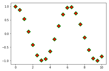
Параметр Тип Описание x array_like, shape (n, ) Набор данных для оси абсцисс y array_like, shape (n, ) Набор данных для оси ординат s scalar или array_like, shape (n, ), optional Масштаб точек c color, sequence, или sequence of color, optional Цвет marker MarkerStyle , optional Стиль точки объекта cmap Colormap , optional, default: None Цветовая схема norm Normalize , optional, default: None Нормализация данных alpha scalar, optional, default: None Прозрачность linewidths scalar или array_like, optional, default: None Ширина границы маркера edgecolors или color или sequence of color, optional. Цвет границы Создадим решение, использующее расширенные параметры для настройки отображения графика:
x = np.arange(0, 10.5, 0.5) y = np.cos(x) plt.scatter(x, y, s=80, c="r", marker="D", linewidths=2, edgecolors="g")
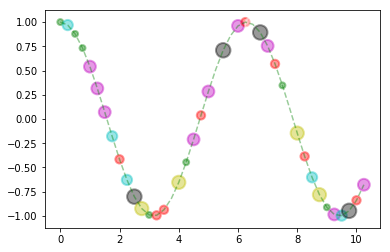
Пример, демонстрирующий работу с цветом и размером:
import matplotlib.colors as mcolors bc = mcolors.BASE_COLORS x = np.arange(0, 10.5, 0.25) y = np.cos(x) num_set = np.random.randint(1, len(mcolors.BASE_COLORS), len(x)) sizes = num_set * 35 colors = [list(bc.keys())[i] for i in num_set] plt.scatter(x, y, s=sizes, alpha=0.4, c=colors, linewidths=2, edgecolors="face") plt.plot(x, y, "g--", alpha=0.4)
Статьи с описанием различных вариантов работы с точечными графиками
P.S.
Вводные уроки по “Линейной алгебре на Python” вы можете найти соответствующей странице нашего сайта . Все уроки по этой теме собраны в книге “Линейная алгебра на Python”.
Если вам интересна тема анализа данных, то мы рекомендуем ознакомиться с библиотекой Pandas. Для начала вы можете познакомиться с вводными уроками. Все уроки по библиотеке Pandas собраны в книге “Pandas. Работа с данными”.
Matplotlib. Урок 4.2. Визуализация данных. Ступенчатый, стековый, точечный график и другие : 1 комментарий
Plot types#
Overview of many common plotting commands in Matplotlib.
Note that we have stripped all labels, but they are present by default. See the gallery for many more examples and the tutorials page for longer examples.
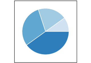
Basic#
Basic plot types, usually y versus x.
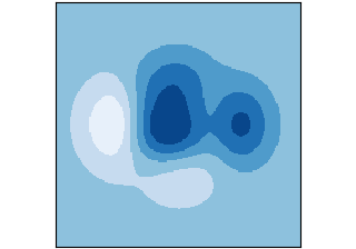
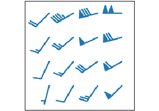
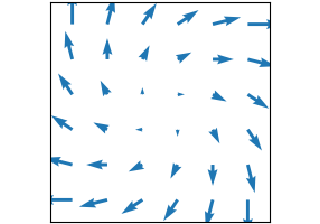
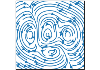
Plots of arrays and fields#
Plotting for arrays of data Z(x, y) and fields U(x, y), V(x, y) .
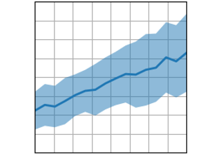
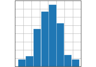
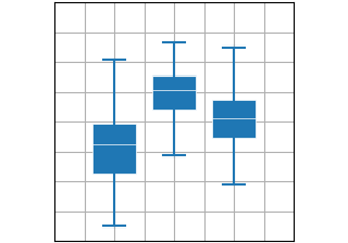
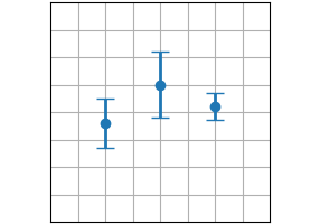
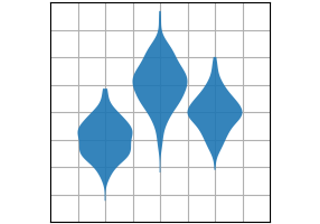
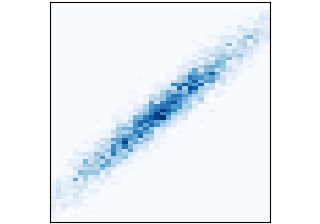
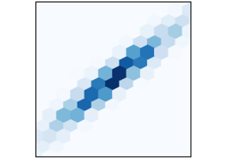
Statistics plots#
Plots for statistical analysis.
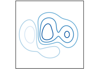
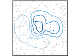
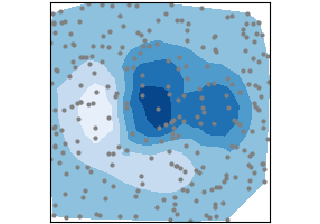
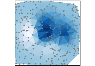
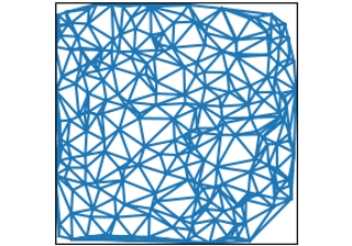
Unstructured coordinates#
Sometimes we collect data z at coordinates (x,y) and want to visualize as a contour. Instead of gridding the data and then using contour , we can use a triangulation algorithm and fill the triangles.
3D#
3D plots using the mpl_toolkits.mplot3d library.