Librosa play audio python

An introduction to libROSA for working with audio

Librosa is powerful Python library built to work with audio and perform analysis on it. It is the starting point towards working with audio data at scale for a wide range of applications such as detecting voice from a person to finding personal characteristics from an audio.

In this article, we will learn:

• how to use Librosa and load an audio file into it
• Get audio timeline, plot it for amplitude, find tempo and pitch
• Compute mel-scaled spectrogram, time stretch an audio, remix an audio

• Audio signal analysis for music.
• Reference implementation of common methods.
• Building blocks for Music information retrieval (MIR).

For a better understanding of libROSA it is said to have a knowledge about NumPy and SciPy.

libROSA can be defined as a package which is structured as collection of submodules which further contains other functions.

For installing the libROSA you just need to run the following command in your command line:

In your Python code, you can import it as:

We will use Matplotlib library for plotting the results and Numpy library to handle the data as array.

Loading your audio file :

The first step towards our analysis is to load an audio library into our code. This is done using librosa.core.load() function. Audio will be automatically resampled to the given rate (default = 22050). To preserve the native sampling rate of the file, use sr=None.

librosa.core.load(path, sr=22050, mono=True, offset=0.0, duration=None, dtype=, res_type='kaiser_best') 

Any codec supported by soundfile or audioread will work. If the codec is supported by soundfile, then path can also be an open file descriptor (int), or any object implementing Python’s file interface. If the codec is not supported by soundfile (e.g., MP3), then only string file paths are supported.

• sr is the sampling rate
• mono is the option (true/ false) to convert it into mono file.
• offset is a floating point number which is the starting time to read the file
• duration is a floating point number which signifies how much of the file to load.
• dtype is the numeric representation of data can be float32, float16, int8 and others.
• res_type is the type of resampling (one option is kaiser_best)

Timeline for your audio

In this code, we will print the timeline of the audio file. We will simply load the audio, convert it into a numpy array and print the output for one sample (by dividing by sampling rate).

import numpy as np import matplotlib.pyplot as plt from glob import glob import librosa as lr audio='arabic6' # change with the name of your audio y, sr = lr.load('./<>.wav'.format(audio)) #you just need to make sure your audio is in the same folder in which you are coding or else you can change the path as per your requirement time = np.arange(0,len(y))/sr print(time) # prints timeline of arabic6 

[0.00000000e+00 4.53514739e-05 9.07029478e-05 . 2.63027211e+01 2.63027664e+01 2.63028118e+01] 

Plotting the audio :

Plotting the audio as Time v/s Sound amplitude

import numpy as np import matplotlib.pyplot as plt from glob import glob import librosa as lr audio='arabic6' y, sr = lr.load('./<>.wav'.format(audio)) time = np.arange(0,len(y))/sr fig, ax = plt.subplots() ax.plot(time,y) ax.set(xlabel='Time(s)',ylabel='sound amplitude') plt.show()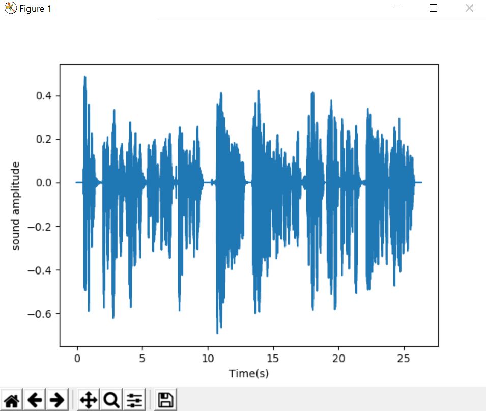 

Plotting and finding the estimating tempo

Tempo was originally used to describe the timing of music, or the speed at which a piece of music is played or can be defined as beats per second.

librosa.beat.tempo(y=None, sr=22050, onset_envelope=None, hop_length=512, start_bpm=120, std_bpm=1.0, ac_size=8.0, max_tempo=320.0, aggregate=) 

It will return tempo as an array

• y: audio time series
• sr: sampling rate of the time series
• onset_envelope: pre-computed onset strength envelope
• hop_length: hop length of the time series
• start_bpm: initial guess of the BPM
• std_bpm: standard deviation of tempo distribution
• ac_size: length (in seconds) of the auto-correlation window
• max_tempo: estimate tempo below this threshold
• aggregate: for estimating global tempo. If None, then tempo is estimated independently for each frame.

CODE

import numpy as np import matplotlib.pyplot as plt from glob import glob import librosa as lr audio='arabic6' y, sr = lr.load('./<>.wav'.format(audio)) onset_env = lr.onset.onset_strength(y, sr=sr) tempo = lr.beat.tempo(onset_envelope=onset_env, sr=sr) print(tempo) tempo = np.asscalar(tempo) # Compute 2-second windowed autocorrelation hop_length = 512 ac = lr.autocorrelate(onset_env, 2 * sr // hop_length) freqs = lr.tempo_frequencies(len(ac), sr=sr,hop_length=hop_length) # Plot on a BPM axis. We skip the first (0-lag) bin. plt.figure(figsize=(8,4)) plt.semilogx(freqs[1:], lr.util.normalize(ac)[1:],label='Onset autocorrelation', basex=2) plt.axvline(tempo, 0, 1, color='r', alpha=0.75, linestyle='--',label='Tempo: BPM'.format(tempo)) plt.xlabel('Tempo (BPM)') plt.grid() plt.title('Static tempo estimation') plt.legend(frameon=True) plt.axis('tight') plt.show()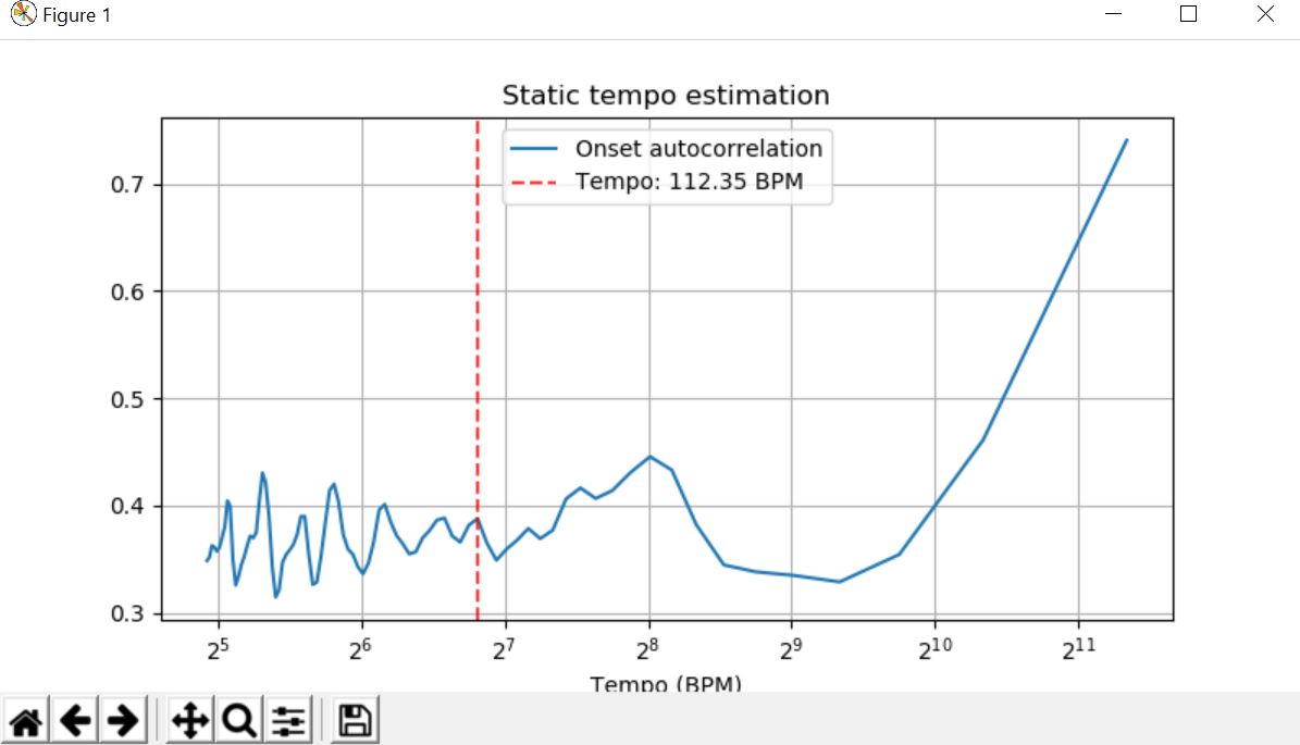 

Finding and plotting the pitch

The sensation of a frequency is commonly referred to as the pitch of a sound. A high pitch sound corresponds to a high frequency sound wave and a low pitch sound corresponds to a low frequency sound wave.

librosa.core.piptrack(y=None, sr=22050, S=None, n_fft=2048, hop_length=None, fmin=150.0, fmax=4000.0, threshold=0.1, win_length=None, window='hann', center=True, pad_mode='reflect', ref=None) 

• y: audio signal
• sr: audio sampling rate of y
• S: magnitude or power spectrogram
• n_fft: number of FFT bins to use, if y is provided.
• hop_length: number of samples to hop
• threshold: A bin in spectrum S is considered a pitch when it is greater than threshold * ref(S).
• fmin: lower frequency cutoff.
• fmax: upper frequency cutoff.
• win_length: Each frame of audio is windowed by window().
• ref:scalar or callable for pitch

• pitches:np.ndarray [shape=(d, t)]
• magnitudes:np.ndarray [shape=(d,t)]
  Where d is the subset of FFT bins within fmin and fmax.

pitches[f, t] contains instantaneous frequency at bin f, time t

magnitudes[f, t] contains the corresponding magnitudes.

Both pitches and magnitudes take value 0 at bins of non-maximal magnitude.

CODE

import numpy as np import matplotlib.pyplot as plt from glob import glob import librosa as lr from IPython.display import Audio audio='arabic6' y, sr = lr.load('./<>.wav'.format(audio)) pitches, magnitudes = lr.piptrack(y=y, sr=sr) print(pitches) print('///') print(magnitudes) plt.subplot(212) plt.show() plt.plot(pitches) plt.show() 

[[0. 0. 0. . 0. 0. 0.] [0. 0. 0. . 0. 0. 0.] [0. 0. 0. . 0. 0. 0.] . [0. 0. 0. . 0. 0. 0.] [0. 0. 0. . 0. 0. 0.] [0. 0. 0. . 0. 0. 0.]] /// [[0. 0. 0. . 0. 0. 0.] [0. 0. 0. . 0. 0. 0.] [0. 0. 0. . 0. 0. 0.] . [0. 0. 0. . 0. 0. 0.] [0. 0. 0. . 0. 0. 0.] [0. 0. 0. . 0. 0. 0.]] 

Compute a mel-scaled spectrogram

An object of type MelSpectrogram represents an acoustic time-frequency representation of a sound

librosa.feature.melspectrogram(y=None, sr=22050, S=None, n_fft=2048, hop_length=512, win_length=None, window='hann', center=True, pad_mode='reflect', power=2.0, **kwargs) 

Parammeters :

• y: audio time-series
• sr: sampling rate of y
• S: spectrogram
• n_fft: length of the FFT window
• hop_length: number of samples between successive frames. See librosa.core.stft
• win_length: Each frame of audio is windowed by window().
• power: Exponent for the magnitude melspectrogram. e.g., 1 for energy, 2 for power, etc.
• kwargs:additional keyword arguments
  Mel filter bank parameters. See librosa.filters.mel for details.

CODE

import numpy as np import matplotlib.pyplot as plt from glob import glob import librosa as lr import librosa.display audio='arabic6' y, sr = lr.load('./<>.wav'.format(audio)) lr.feature.melspectrogram(y=y, sr=sr) D = np.abs(lr.stft(y))**2 S = lr.feature.melspectrogram(S=D) S = lr.feature.melspectrogram(y=y, sr=sr, n_mels=128,fmax=8000) plt.figure(figsize=(10, 4)) lr.display.specshow(lr.power_to_db(S,ref=np.max),y_axis='mel', fmax=8000,x_axis='time') plt.colorbar(format='%+2.0f dB') plt.title('Mel spectrogram') plt.tight_layout() plt.show()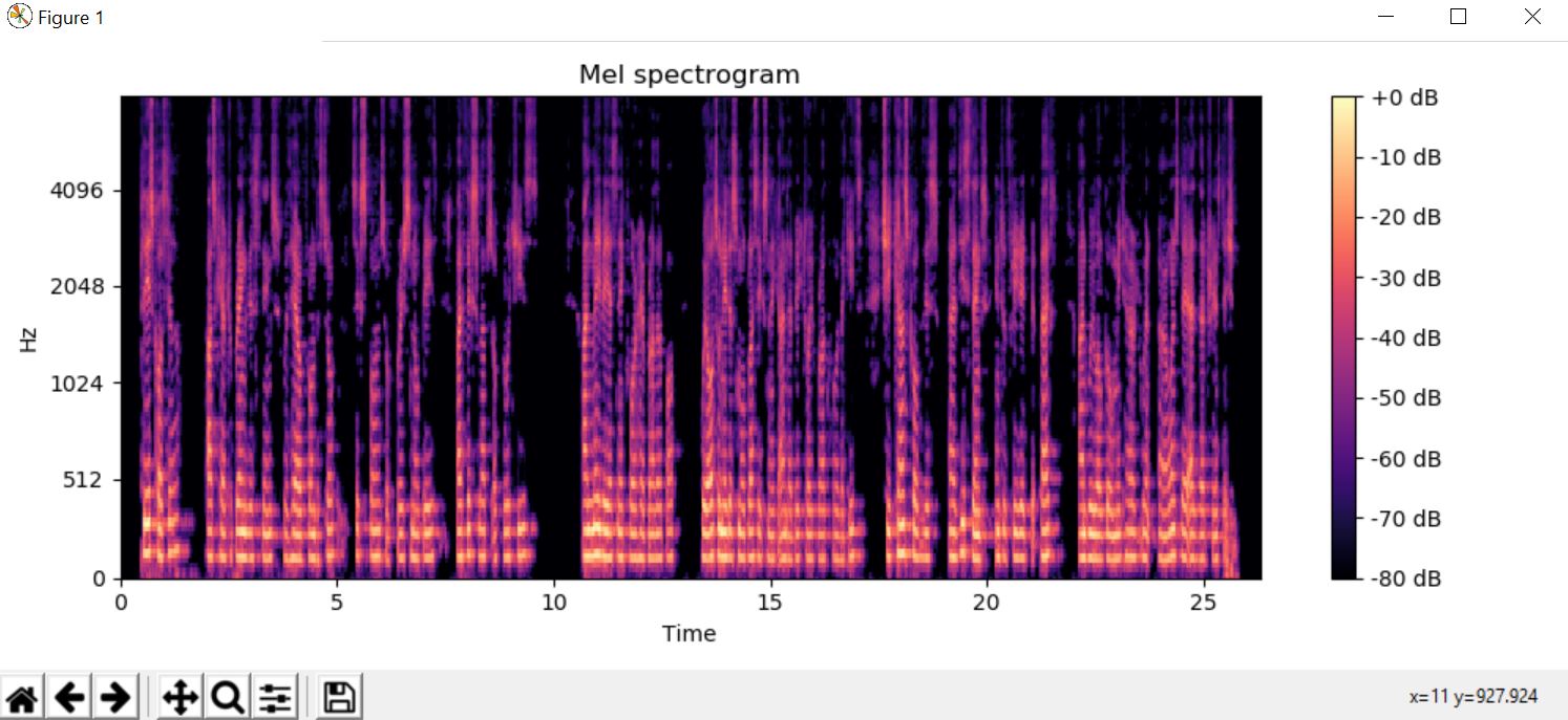 

Output :

Modifying the audio :

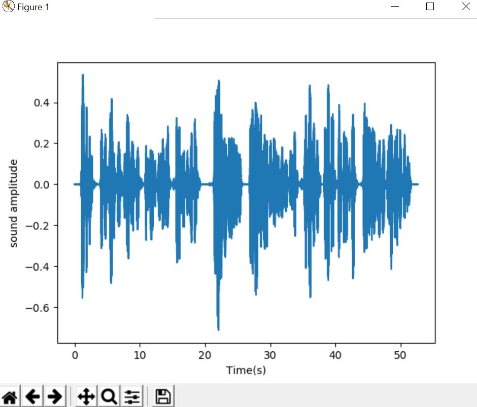
Time-stretch an audio series by a fixed rate

librosa.effects.time_stretch(y, rate, **kwargs) 

• y: audio time series
• rate: Stretch factor. If rate > 1, then the signal is sped up. If rate < 1, then the signal is slowed down.
• kwargs: additional keyword arguments.
  See librosa.decompose.stft for details.

CODE

import numpy as np import matplotlib.pyplot as plt from glob import glob import librosa as lr audio='arabic6' y, sr = lr.load('./<>.wav'.format(audio)) y_fast = lr.effects.time_stretch(y, 2.0) time = np.arange(0,len(y_fast))/sr fig, ax = plt.subplots() ax.plot(time,y_fast) ax.set(xlabel='Time(s)',ylabel='sound amplitude') plt.show()#compress to be twice as fast y_slow = lr.effects.time_stretch(y, 0.5) time = np.arange(0,len(y_slow))/sr fig, ax = plt.subplots() ax.plot(time,y_slow) ax.set(xlabel='Time(s)',ylabel='sound amplitude') plt.show()#half the original speed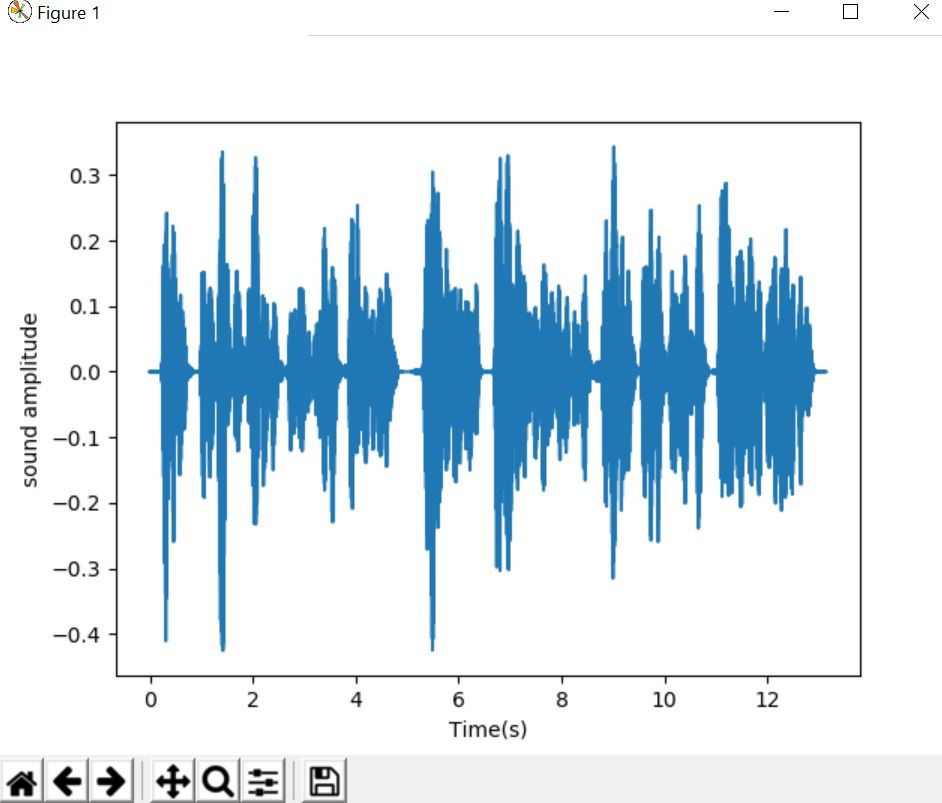 

Remix an audio signal by re-ordering time intervals

Remix is a piece of media which has been altered from its original state by adding, removing and changing pieces of the item. A song, piece of artwork, books, video, or photograph can all be remixes. The only characteristic of a remix is that it appropriates and changes other materials to create something new.

librosa.effects.remix(y, intervals, align_zeros=True) 

Parameters :

• y: Audio time series
• intervals: iterable of tuples (start, end)
  An iterable (list-like or generator) where the i th item intervals[i] indicates the start and end (in samples) of a slice of y.
• align_zeros: boolean
  If True, interval boundaries are mapped to the closest zero-crossing in y. If y is stereo, zero-crossings are computed after converting to mono.

CODE

import numpy as np import matplotlib.pyplot as plt from glob import glob import librosa as lr audio='arabic6' y, sr = lr.load('./<>.wav'.format(audio)) _, beat_frames = lr.beat.beat_track(y=y, sr=sr,hop_length=512) beat_samples = lr.frames_to_samples(beat_frames) intervals = lr.util.frame(beat_samples, frame_length=2,hop_length=1).T y_out = lr.effects.remix(y, intervals[::-1]) time = np.arange(0,len(y_out))/sr fig, ax = plt.subplots() ax.plot(time,y_out) ax.set(xlabel='Time(s)',ylabel='sound amplitude') plt.show()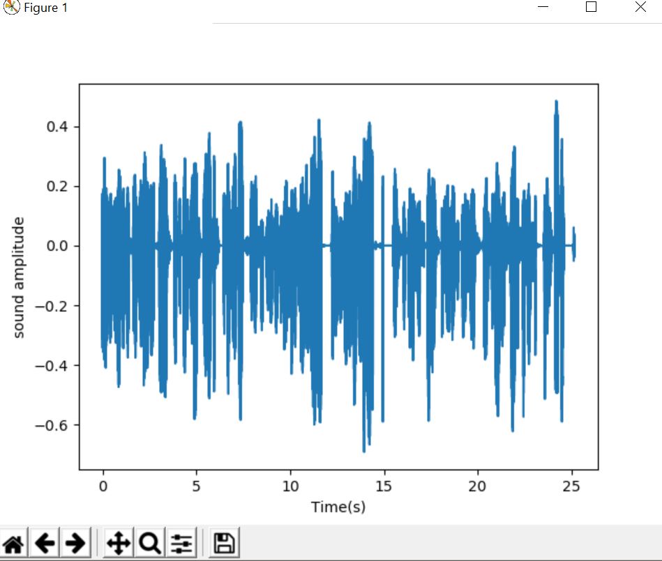 

Harshita Sahai

Maintainer at OpenGenus | Previously Software Developer, Intern at OpenGenus (June to August 2019) | B.Tech in Information Technology from Guru Gobind Singh Indraprastha University (2017 to 2021)

OpenGenus Tech Review Team

Software Engineering

Understand Neural Networks intuitively

Neural Networks act as a ‘black box’ that takes inputs and predicts an output and it learns complex non-linear mappings to produce far more accurate output classification results.

Yashwant Saini

Introduction to Mongoose and how to work with MongoDb with Mongoose

In this article, we will explore Mongoose and get an idea of using it with MongoDB through a demo. We will learn how to create, update, delete and read documents in MongoDB.

Priyanka Yadav

Источник