Divide and conquer python

Divide and Conquer Algorithms in Python

Hello there programmers, I am Aditya, back again with another article on python. In this blog post, we’re going to dive into the world of Divide and Conquer — a powerful strategy for tackling complex problems. We’ll break down the key principles behind Divide and Conquer and explore some fun and useful examples that will have you feeling like a problem-solving pro in no time! Whether you’re a seasoned programmer or just starting out, this post is your ticket to mastering Divide and Conquer and taking your problem-solving skills to the next level. So grab a cup of coffee (or your beverage of choice) and let’s get started!»

Introduction to Divide and Conquer Algorithm

Divide and conquer is a popular algorithmic paradigm that involves breaking down a problem into smaller, more manageable sub-problems, solving each sub-problem independently, and then combining the solutions to the sub-problems to produce the final solution to the original problem.

3 key steps of Divide and Conquer Algorithm

1. Divide: The problem is divided into smaller sub-problems that can be solved independently. This step usually involves breaking the problem into two or more sub-problems of roughly equal size.
2. Conquer: Each sub-problem is solved independently using recursion or other techniques. This step is where the actual work is done to solve the problem.
3. Combine: The solutions to the sub-problems are combined to form the solution to the original problem. This step usually involves merging the solutions to the sub-problems together.

Applications of Divide and Conquer Algorithm

Divide and Conquer is a versatile problem-solving strategy that can be applied to many different types of problems. Here are some common applications of Divide and Conquer:

Binary Search

Binary Search is a search algorithm that is used to find the position of a target value within a sorted array. The algorithm works by repeatedly dividing the search interval in half until the target value is found. Here’s how Binary Search works:

1. Divide: The search interval is divided in half.
2. Conquer: The algorithm checks whether the target value is in the left or right half of the search interval, and discards the other half.
3. Combine: The algorithm repeats the process on the remaining half until the target value is found or the search interval is empty.

def binary_search(arr, x): low = 0 high = len(arr) - 1 while low  high: mid = (low + high) // 2 if arr[mid] == x: return mid elif arr[mid]  x: low = mid + 1 else: high = mid - 1 return -1 

Binary Search has a time complexity of O(log n), making it a very efficient algorithm for searching sorted arrays.

Merge Sort

Merge Sort is a sorting algorithm that works by repeatedly dividing the input array into two halves, sorting each half separately, and then merging the sorted halves back together. Here’s how Merge Sort works:

1. Divide: The input array is divided in half.
2. Conquer: Recursively sort each half of the input array using Merge Sort.
3. Combine: Merge the sorted halves back together to obtain the final sorted array.

def merge_sort(arr): if len(arr)  1: return arr mid = len(arr) // 2 left = arr[:mid] right = arr[mid:] left = merge_sort(left) right = merge_sort(right) return merge(left, right) 

Merge Sort has a time complexity of O(n log n), making it one of the most efficient sorting algorithms.

Quick Sort

Quick Sort is another sorting algorithm that works by dividing the input array into two partitions, one with elements smaller than a pivot element, and another with elements larger than the pivot element. Here’s how Quick Sort works:

1. Divide: Choose a pivot element and divide the input array into two partitions based on the pivot element.
2. Conquer: Recursively sort each partition using Quick Sort.
3. Combine: Combine the sorted partitions to obtain the final sorted array.

def quick_sort(arr): if len(arr)  1: return arr pivot = arr[len(arr) // 2] left = [x for x in arr if x  pivot] middle = [x for x in arr if x == pivot] right = [x for x in arr if x > pivot] return quick_sort(left) + middle + quick_sort(right) 

Quick Sort has a time complexity of O(n log n) on average, but can have a worst-case time complexity of O(n^2) in certain cases.

Maximum Subarray Sum

The Maximum Subarray Sum problem involves finding the contiguous subarray within a one-dimensional array of numbers that has the largest sum. Here’s how this problem can be solved using Divide and Conquer:

1. Divide: The array is divided in half.
2. Conquer: Recursively find the maximum subarray sum in the left and right sub-arrays.
3. Combine: Calculate the maximum subarray sum that includes the middle element and return the maximum of the three sums.

def max_subarray_sum(arr): if len(arr) == 1: return arr[0] mid = len(arr) // 2 left_max = max_subarray_sum(arr[:mid]) right_max = max_subarray_sum(arr[mid:]) cross_max = max_crossing_sum(arr, mid) return max(left_max, right_max, cross_max) def max_crossing_sum(arr, mid): left_sum = float('-inf') temp_sum = 0 for i in range(mid - 1, -1, -1): temp_sum += arr[i] left_sum = max(left_sum, temp_sum) right_sum = float('-inf') temp_sum = 0 for i in range(mid, len(arr)): temp_sum += arr[i] right_sum = max(right_sum, temp_sum) return left_sum + right_sum 

The time complexity of Maximum Subarray Sum using Divide and Conquer is O(n log n).

Overall, the Divide and Conquer algorithm is a powerful tool that can be used to solve a wide variety of problems. By understanding the basic principles and applications of Divide and Conquer, you can tackle complex problems more efficiently and effectively.

FAANG Interview Question solved using Divide and Conquer Algorithm

Question: Given an unsorted array of integers, find the maximum sum of any contiguous subarray of the array.

Example: For the input array [2, -3, 1, 5, -6, 9], the contiguous subarray with the maximum sum is [1, 5, -6, 9], and the maximum sum is 9 + (-6) + 5 + 1 = 9.

Solution: This problem can be solved efficiently using the Divide and Conquer algorithm. We can recursively divide the input array into two halves, and find the maximum subarray sum in each half.

• The maximum subarray sum in the left half, right half, and the combined subarray containing the middle element can be computed in constant time.
• The maximum subarray sum in the combined subarray can be computed by finding the maximum subarray sum starting from the middle element, and the maximum subarray sum ending at the middle element, and adding them together. This can also be done in linear time.
• Here’s the Python code to solve the problem using the Divide and Conquer algorithm:

def max_subarray_sum(arr): if len(arr) == 1: return arr[0] mid = len(arr) // 2 left_sum = max_subarray_sum(arr[:mid]) right_sum = max_subarray_sum(arr[mid:]) # find the maximum subarray sum starting from the middle element left_max = arr[mid-1] temp_sum = 0 for i in range(mid-1, -1, -1): temp_sum += arr[i] left_max = max(left_max, temp_sum) # find the maximum subarray sum ending at the middle element right_max = arr[mid] temp_sum = 0 for i in range(mid, len(arr)): temp_sum += arr[i] right_max = max(right_max, temp_sum) # return the maximum subarray sum in the left half, right half, or combined subarray return max(left_sum, right_sum, left_max + right_max) 

Resources

To further your learning and practice of Divide and Conquer algorithms in Python, I recommend exploring some of these resources and trying out some of the practice problems and exercises they offer.

As you gain more experience with these algorithms, you can start to apply them to real-world problems and see the benefits of using this approach to problem-solving.

There are many resources available for learning and practicing Divide and Conquer algorithms in Python, including Python Algorithm Visualization (PAV), GeeksforGeeks, HackerRank, Coursera, and Codecademy.

Conclusion

And that, my friends, concludes our journey into the wonderful world of Divide and Conquer algorithms! We’ve explored the basics, dug into some key applications, and even written some code to solve a classic interview question.

So, as we wrap up this blog post, I’d like to leave you with one final thought: the next time you’re faced with a challenging problem, remember the power of Divide and Conquer algorithms. By breaking it down into smaller, more manageable subproblems, you can find an elegant solution that will make you feel like a true coding wizard!

Источник

Divide and Conquer Algorithm

In this tutorial, you will learn how the divide and conquer algorithm works. We will also compare the divide and conquer approach versus other approaches to solve a recursive problem.

A divide and conquer algorithm is a strategy of solving a large problem by

1. breaking the problem into smaller sub-problems
2. solving the sub-problems, and
3. combining them to get the desired output.

To use the divide and conquer algorithm, recursion is used. Learn about recursion in different programming languages:

How Divide and Conquer Algorithms Work?

Here are the steps involved:

1. Divide: Divide the given problem into sub-problems using recursion.
2. Conquer: Solve the smaller sub-problems recursively. If the subproblem is small enough, then solve it directly.
3. Combine: Combine the solutions of the sub-problems that are part of the recursive process to solve the actual problem.

Let us understand this concept with the help of an example.

Here, we will sort an array using the divide and conquer approach (ie. merge sort).

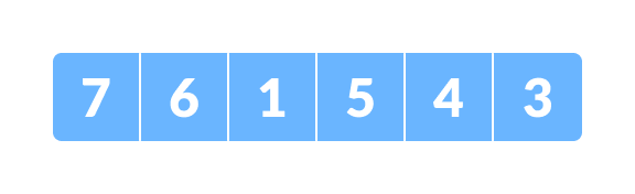
1. Let the given array be:
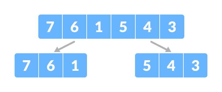
2. Divide the array into two halves.
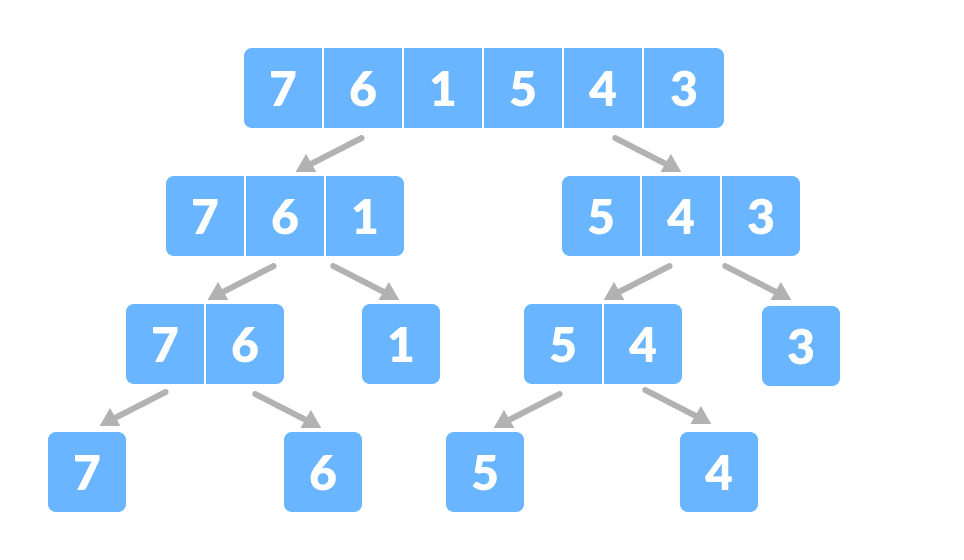
   Again, divide each subpart recursively into two halves until you get individual elements.
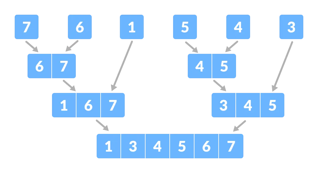
3. Now, combine the individual elements in a sorted manner. Here, conquer and combine steps go side by side.

Time Complexity

The complexity of the divide and conquer algorithm is calculated using the master theorem.

T(n) = aT(n/b) + f(n), where, n = size of input a = number of subproblems in the recursion n/b = size of each subproblem. All subproblems are assumed to have the same size. f(n) = cost of the work done outside the recursive call, which includes the cost of dividing the problem and cost of merging the solutions

Let us take an example to find the time complexity of a recursive problem.

For a merge sort, the equation can be written as:

T(n) = aT(n/b) + f(n) = 2T(n/2) + O(n) Where, a = 2 (each time, a problem is divided into 2 subproblems) n/b = n/2 (size of each sub problem is half of the input) f(n) = time taken to divide the problem and merging the subproblems T(n/2) = O(n log n) (To understand this, please refer to the master theorem.) Now, T(n) = 2T(n log n) + O(n) ≈ O(n log n)

Divide and Conquer Vs Dynamic approach

The divide and conquer approach divides a problem into smaller subproblems; these subproblems are further solved recursively. The result of each subproblem is not stored for future reference, whereas, in a dynamic approach, the result of each subproblem is stored for future reference.

Use the divide and conquer approach when the same subproblem is not solved multiple times. Use the dynamic approach when the result of a subproblem is to be used multiple times in the future.

Let us understand this with an example. Suppose we are trying to find the Fibonacci series. Then,

Divide and Conquer approach:

Dynamic approach:

mem = [] fib(n) If n in mem: return mem[n] else, If n < 2, f = 1 else , f = f(n - 1) + f(n -2) mem[n] = f return f

In a dynamic approach, mem stores the result of each subproblem.

Advantages of Divide and Conquer Algorithm

• The complexity for the multiplication of two matrices using the naive method is O(n 3 ) , whereas using the divide and conquer approach (i.e. Strassen's matrix multiplication) is O(n 2.8074 ) . This approach also simplifies other problems, such as the Tower of Hanoi.
• This approach is suitable for multiprocessing systems.
• It makes efficient use of memory caches.

Divide and Conquer Applications

Table of Contents

Free Courses on YouTube

Python Full Course Playlist
105 STL Algorithms in Less Than an Hour
C++ STL Playlist
Learn Node.js
Learn Data Science Full course
Learn Computer Networking Full course

Источник