Binary classification in python

Binary Classification

In machine learning, binary classification is a supervised learning algorithm that categorizes new observations into one of two classes.

The following are a few binary classification applications, where the 0 and 1 columns are two possible classes for each observation:

Application	Observation	0	1
Medical Diagnosis	Patient	Healthy	Diseased
Email Analysis	Email	Not Spam	Spam
Financial Data Analysis	Transaction	Not Fraud	Fraud
Marketing	Website visitor	Won’t Buy	Will Buy
Image Classification	Image	Hotdog	Not Hotdog

Quick example

In a medical diagnosis, a binary classifier for a specific disease could take a patient’s symptoms as input features and predict whether the patient is healthy or has the disease. The possible outcomes of the diagnosis are positive and negative.

Evaluation of binary classifiers

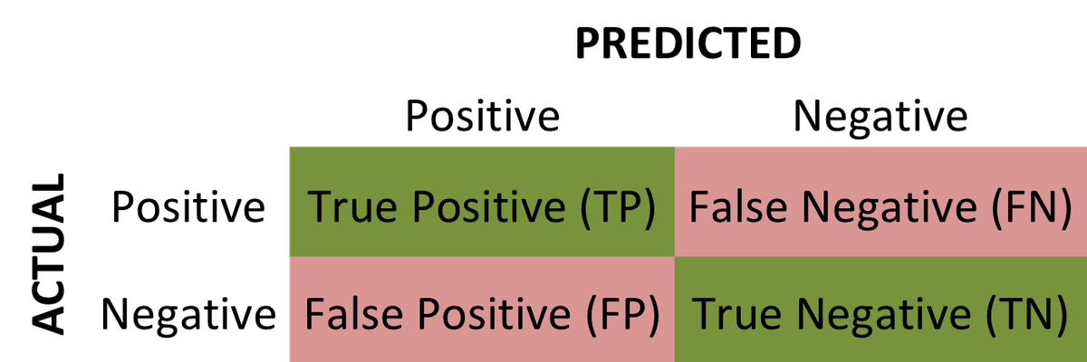
If the model successfully predicts the patients as positive, this case is called True Positive (TP). If the model successfully predicts patients as negative, this is called True Negative (TN). The binary classifier may misdiagnose some patients as well. If a diseased patient is classified as healthy by a negative test result, this error is called False Negative (FN). Similarly, If a healthy patient is classified as diseased by a positive test result, this error is called False Positive(FP).

We can evaluate a binary classifier based on the following parameters:

• True Positive (TP): The patient is diseased and the model predicts «diseased»
• False Positive (FP): The patient is healthy but the model predicts «diseased»
• True Negative (TN): The patient is healthy and the model predicts «healthy»
• False Negative (FN): The patient is diseased and the model predicts «healthy»

After obtaining these values, we can compute the accuracy score of the binary classifier as follows: $$ accuracy = \frac $$

The following is a confusion matrix, which represents the above parameters:

In machine learning, many methods utilize binary classification. The most common are:

• Support Vector Machines
• Naive Bayes
• Nearest Neighbor
• Decision Trees
• Logistic Regression
• Neural Networks

The following Python example will demonstrate using binary classification in a logistic regression problem.

A Python example for binary classification

For our data, we will use the breast cancer dataset from scikit-learn. This dataset contains tumor observations and corresponding labels for whether the tumor was malignant or benign.

First, we’ll import a few libraries and then load the data. When loading the data, we’ll specify as_frame=True so we can work with pandas objects (see our pandas tutorial for an introduction).

The dataset contains a DataFrame for the observation data and a Series for the target data.

Let’s see what the first few rows of observations look like:

mean radius	mean texture	mean perimeter	mean area	mean smoothness	mean compactness	mean concavity	mean concave points	mean symmetry	mean fractal dimension	.	worst radius	worst texture	worst perimeter	worst area	worst smoothness	worst compactness	worst concavity	worst concave points	worst symmetry	worst fractal dimension
0	17.99	10.38	122.80	1001.0	0.11840	0.27760	0.3001	0.14710	0.2419	0.07871	.	25.38	17.33	184.60	2019.0	0.1622	0.6656	0.7119	0.2654	0.4601	0.11890
1	20.57	17.77	132.90	1326.0	0.08474	0.07864	0.0869	0.07017	0.1812	0.05667	.	24.99	23.41	158.80	1956.0	0.1238	0.1866	0.2416	0.1860	0.2750	0.08902
2	19.69	21.25	130.00	1203.0	0.10960	0.15990	0.1974	0.12790	0.2069	0.05999	.	23.57	25.53	152.50	1709.0	0.1444	0.4245	0.4504	0.2430	0.3613	0.08758
3	11.42	20.38	77.58	386.1	0.14250	0.28390	0.2414	0.10520	0.2597	0.09744	.	14.91	26.50	98.87	567.7	0.2098	0.8663	0.6869	0.2575	0.6638	0.17300
4	20.29	14.34	135.10	1297.0	0.10030	0.13280	0.1980	0.10430	0.1809	0.05883	.	22.54	16.67	152.20	1575.0	0.1374	0.2050	0.4000	0.1625	0.2364	0.07678

The output shows five observations with a column for each feature we’ll use to predict malignancy.

The targets for the first five observations are all zero, meaning the tumors are benign. Here’s how many malignant and benign tumors are in our dataset:

So we have 357 malignant tumors, denoted as 1, and 212 benign, denoted as 0. So, we have a binary classification problem.

To perform binary classification using logistic regression with sklearn, we must accomplish the following steps.

Step 1: Define explanatory and target variables

We’ll store the rows of observations in a variable X and the corresponding class of those observations (0 or 1) in a variable y .

Step 2: Split the dataset into training and testing sets

We use 75% of data for training and 25% for testing. Setting random_state=0 will ensure your results are the same as ours.

Step 3: Normalize the data for numerical stability

Note that we normalize after splitting the data. It’s good practice to apply any data transformations to training and testing data separately to prevent data leakage.

Step 4: Fit a logistic regression model to the training data

This step effectively trains the model to predict the targets from the data.

Step 5: Make predictions on the testing data

With the model trained, we now ask the model to predict targets based on the test data.

Step 6: Calculate the accuracy score by comparing the actual values and predicted values.

We can now calculate how well the model performed by comparing the model’s predictions to the true target values, which we reserved in the y_test variable.

First, we’ll calculate the confusion matrix to get the necessary parameters:

With these values, we can now calculate an accuracy score:

Other binary classifiers in the scikit-learn library

Logistic regression is just one of many classification algorithms defined in Scikit-learn. We’ll compare several of the most common, but feel free to read more about these algorithms in the sklearn docs here.

We’ll also use the sklearn Accuracy, Precision, and Recall metrics for performance evaluation. See the docs here if you’d like to read more about the available metrics.

Initializing each binary classifier

To quickly train each model in a loop, we’ll initialize each model and store it by name in a dictionary:

Performance evaluation of each binary classifier

Now that we’veinitialized the models, we’ll loop over each one, train it by calling .fit() , make predictions, calculate metrics, and store each result in a dictionary.

With all metrics stored, we can use pandas to view the data as a table:

Accuracy	Precision	Recall
Logistic Regression	0.958042	0.955556	0.977273
Support Vector Machines	0.937063	0.933333	0.965517
Decision Trees	0.902098	0.866667	0.975000
Random Forest	0.972028	0.966667	0.988636
Naive Bayes	0.937063	0.955556	0.945055
K-Nearest Neighbor	0.951049	0.988889	0.936842

Finally, here’s a quick bar chart to compare the classifiers’ performance:

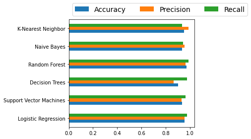
Since we’re only using the default model parameters, we won’t know which classifier is better. We should optimize each algorithm’s parameters first to know which one has the best performance.

Источник

Beginner’s Project on Binary Classification in Python – Sonar Dataset

Binary Classification is a type of machine learning problem where the goal is to classify instances into one of two classes. The Sonar Dataset is a popular dataset for binary classification problems, which is used to distinguish between metal cylinders and rocks from a sonar return signal.

The Sonar dataset includes 208 observations, each of which has 60 input features and one binary output variable (R or M). The input features represent different characteristics of the sonar return signal, such as the frequency and the time of the echoes. The output variable indicates whether the observation represents a rock or a metal cylinder.

There are several algorithms that can be used for binary classification in Python, such as logistic regression, decision trees, and support vector machines (SVMs). These algorithms can be implemented using libraries such as scikit-learn.

When working with the Sonar dataset, it’s important to preprocess the data by normalizing the input features. This can help to avoid numerical instability and improve the performance of the classifier.

Once the data is ready, the next step is to split the data into training and testing sets. The training set is used to train the classifier, and the testing set is used to evaluate its performance.

After that, the classifier can be trained using the training set and the chosen algorithm. Once the classifier is trained, it can be used to make predictions on the testing set. This will give an estimate of the classifier’s performance on unseen data.

Finally, the model can be improved by trying different algorithms, tuning the hyperparameters, or by using techniques like cross-validation.

In summary, Binary Classification is a type of machine learning problem where the goal is to classify instances into one of two classes. The Sonar dataset is a popular dataset for binary classification problems, which is used to distinguish between metal cylinders and rocks from a sonar return signal. There are several algorithms that can be used for binary classification in Python, such as logistic regression, decision trees, and support vector machines (SVMs). When working with the Sonar dataset, it’s important to preprocess the data by normalizing the input features. Once the data is ready, the next step is to split the data into training and testing sets. After that, the classifier can be trained using the training set and the chosen algorithm. Once the classifier is trained, it can be used to make predictions on the testing set. Finally, the model can be improved by trying different algorithms, tuning the hyperparameters, or by using techniques like cross-validation.

In this Applied Machine Learning & Data Science Recipe (Jupyter Notebook), the reader will find the practical use of applied machine learning and data science in Python programming: how to do an end-to-end Beginner’s Project on Binary Classification in Python.

Источник