Special functions ( scipy.special )#
The main feature of the scipy.special package is the definition of numerous special functions of mathematical physics. Available functions include airy, elliptic, bessel, gamma, beta, hypergeometric, parabolic cylinder, mathieu, spheroidal wave, struve, and kelvin. There are also some low-level stats functions that are not intended for general use as an easier interface to these functions is provided by the stats module. Most of these functions can take array arguments and return array results following the same broadcasting rules as other math functions in Numerical Python. Many of these functions also accept complex numbers as input. For a complete list of the available functions with a one-line description type >>> help(special). Each function also has its own documentation accessible using help. If you don’t see a function you need, consider writing it and contributing it to the library. You can write the function in either C, Fortran, or Python. Look in the source code of the library for examples of each of these kinds of functions.
Bessel functions of real order( jv , jn_zeros )#
Bessel functions are a family of solutions to Bessel’s differential equation with real or complex order alpha:
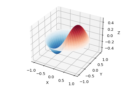
Among other uses, these functions arise in wave propagation problems, such as the vibrational modes of a thin drum head. Here is an example of a circular drum head anchored at the edge:
>>> from scipy import special >>> import numpy as np >>> def drumhead_height(n, k, distance, angle, t): . kth_zero = special.jn_zeros(n, k)[-1] . return np.cos(t) * np.cos(n*angle) * special.jn(n, distance*kth_zero) >>> theta = np.r_[0:2*np.pi:50j] >>> radius = np.r_[0:1:50j] >>> x = np.array([r * np.cos(theta) for r in radius]) >>> y = np.array([r * np.sin(theta) for r in radius]) >>> z = np.array([drumhead_height(1, 1, r, theta, 0.5) for r in radius])
>>> import matplotlib.pyplot as plt >>> fig = plt.figure() >>> ax = fig.add_axes(rect=(0, 0.05, 0.95, 0.95), projection='3d') >>> ax.plot_surface(x, y, z, rstride=1, cstride=1, cmap='RdBu_r', vmin=-0.5, vmax=0.5) >>> ax.set_xlabel('X') >>> ax.set_ylabel('Y') >>> ax.set_xticks(np.arange(-1, 1.1, 0.5)) >>> ax.set_yticks(np.arange(-1, 1.1, 0.5)) >>> ax.set_zlabel('Z') >>> plt.show()
Cython Bindings for Special Functions ( scipy.special.cython_special )#
SciPy also offers Cython bindings for scalar, typed versions of many of the functions in special. The following Cython code gives a simple example of how to use these functions:
cimport scipy.special.cython_special as csc cdef: double x = 1 double complex z = 1 + 1j double si, ci, rgam double complex cgam rgam = csc.gamma(x) print(rgam) cgam = csc.gamma(z) print(cgam) csc.sici(x, &si, &ci) print(si, ci)
(See the Cython documentation for help with compiling Cython.) In the example the function csc.gamma works essentially like its ufunc counterpart gamma , though it takes C types as arguments instead of NumPy arrays. Note, in particular, that the function is overloaded to support real and complex arguments; the correct variant is selected at compile time. The function csc.sici works slightly differently from sici ; for the ufunc we could write ai, bi = sici(x) , whereas in the Cython version multiple return values are passed as pointers. It might help to think of this as analogous to calling a ufunc with an output array: sici(x, out=(si, ci)) .
There are two potential advantages to using the Cython bindings:
- they avoid Python function overhead
- they do not require the Python Global Interpreter Lock (GIL)
The following sections discuss how to use these advantages to potentially speed up your code, though, of course, one should always profile the code first to make sure putting in the extra effort will be worth it.
Avoiding Python Function Overhead#
For the ufuncs in special, Python function overhead is avoided by vectorizing, that is, by passing an array to the function. Typically, this approach works quite well, but sometimes it is more convenient to call a special function on scalar inputs inside a loop, for example, when implementing your own ufunc. In this case, the Python function overhead can become significant. Consider the following example:
import scipy.special as sc cimport scipy.special.cython_special as csc def python_tight_loop(): cdef: int n double x = 1 for n in range(100): sc.jv(n, x) def cython_tight_loop(): cdef: int n double x = 1 for n in range(100): csc.jv(n, x)
On one computer python_tight_loop took about 131 microseconds to run and cython_tight_loop took about 18.2 microseconds to run. Obviously this example is contrived: one could just call special.jv(np.arange(100), 1) and get results just as fast as in cython_tight_loop . The point is that if Python function overhead becomes significant in your code, then the Cython bindings might be useful.
Releasing the GIL#
One often needs to evaluate a special function at many points, and typically the evaluations are trivially parallelizable. Since the Cython bindings do not require the GIL, it is easy to run them in parallel using Cython’s prange function. For example, suppose that we wanted to compute the fundamental solution to the Helmholtz equation:
where \(k\) is the wavenumber and \(\delta\) is the Dirac delta function. It is known that in two dimensions the unique (radiating) solution is
where \(H_0^\) is the Hankel function of the first kind, i.e., the function hankel1 . The following example shows how we could compute this function in parallel:
from libc.math cimport fabs cimport cython from cython.parallel cimport prange import numpy as np import scipy.special as sc cimport scipy.special.cython_special as csc def serial_G(k, x, y): return 0.25j*sc.hankel1(0, k*np.abs(x - y)) @cython.boundscheck(False) @cython.wraparound(False) cdef void _parallel_G(double k, double[. ] x, double[. ] y, double complex[. ] out) nogil: cdef int i, j for i in prange(x.shape[0]): for j in range(y.shape[0]): out[i,j] = 0.25j*csc.hankel1(0, k*fabs(x[i,j] - y[i,j])) def parallel_G(k, x, y): out = np.empty_like(x, dtype='complex128') _parallel_G(k, x, y, out) return out
(For help with compiling parallel code in Cython see here.) If the above Cython code is in a file test.pyx , then we can write an informal benchmark which compares the parallel and serial versions of the function:
import timeit import numpy as np from test import serial_G, parallel_G def main(): k = 1 x, y = np.linspace(-100, 100, 1000), np.linspace(-100, 100, 1000) x, y = np.meshgrid(x, y) def serial(): serial_G(k, x, y) def parallel(): parallel_G(k, x, y) time_serial = timeit.timeit(serial, number=3) time_parallel = timeit.timeit(parallel, number=3) print("Serial method took seconds".format(time_serial)) print("Parallel method took seconds".format(time_parallel)) if __name__ == "__main__": main()
On one quad-core computer the serial method took 1.29 seconds and the parallel method took 0.29 seconds.
Functions not in scipy.special #
Some functions are not included in special because they are straightforward to implement with existing functions in NumPy and SciPy. To prevent reinventing the wheel, this section provides implementations of several such functions, which hopefully illustrate how to handle similar functions. In all examples NumPy is imported as np and special is imported as sc .
def binary_entropy(x): return -(sc.xlogy(x, x) + sc.xlog1py(1 - x, -x))/np.log(2)
A rectangular step function on [0, 1]:
def step(x): return 0.5*(np.sign(x) + np.sign(1 - x))
Translating and scaling can be used to get an arbitrary step function.
def ramp(x): return np.maximum(0, x)
scipy.signal.bessel#
Design an Nth-order digital or analog Bessel filter and return the filter coefficients.
Parameters : N int
Wn array_like
A scalar or length-2 sequence giving the critical frequencies (defined by the norm parameter). For analog filters, Wn is an angular frequency (e.g., rad/s).
For digital filters, Wn are in the same units as fs. By default, fs is 2 half-cycles/sample, so these are normalized from 0 to 1, where 1 is the Nyquist frequency. (Wn is thus in half-cycles / sample.)
The type of filter. Default is ‘lowpass’.
analog bool, optional
When True, return an analog filter, otherwise a digital filter is returned. (See Notes.)
output , optional
Type of output: numerator/denominator (‘ba’), pole-zero (‘zpk’), or second-order sections (‘sos’). Default is ‘ba’.
Critical frequency normalization:
The filter is normalized such that the phase response reaches its midpoint at angular (e.g. rad/s) frequency Wn. This happens for both low-pass and high-pass filters, so this is the “phase-matched” case.
The magnitude response asymptotes are the same as a Butterworth filter of the same order with a cutoff of Wn.
This is the default, and matches MATLAB’s implementation.
The filter is normalized such that the group delay in the passband is 1/Wn (e.g., seconds). This is the “natural” type obtained by solving Bessel polynomials.
The filter is normalized such that the gain magnitude is -3 dB at angular frequency Wn.
The sampling frequency of the digital system.
Numerator (b) and denominator (a) polynomials of the IIR filter. Only returned if output=’ba’ .
z, p, k ndarray, ndarray, float
Zeros, poles, and system gain of the IIR filter transfer function. Only returned if output=’zpk’ .
sos ndarray
Second-order sections representation of the IIR filter. Only returned if output=’sos’ .
Also known as a Thomson filter, the analog Bessel filter has maximally flat group delay and maximally linear phase response, with very little ringing in the step response. [1]
The Bessel is inherently an analog filter. This function generates digital Bessel filters using the bilinear transform, which does not preserve the phase response of the analog filter. As such, it is only approximately correct at frequencies below about fs/4. To get maximally-flat group delay at higher frequencies, the analog Bessel filter must be transformed using phase-preserving techniques.
See besselap for implementation details and references.
The ‘sos’ output parameter was added in 0.16.0.
Thomson, W.E., “Delay Networks having Maximally Flat Frequency Characteristics”, Proceedings of the Institution of Electrical Engineers, Part III, November 1949, Vol. 96, No. 44, pp. 487-490.
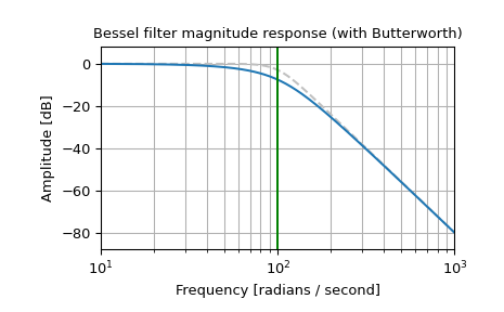
Plot the phase-normalized frequency response, showing the relationship to the Butterworth’s cutoff frequency (green):
>>> from scipy import signal >>> import matplotlib.pyplot as plt >>> import numpy as np
>>> b, a = signal.butter(4, 100, 'low', analog=True) >>> w, h = signal.freqs(b, a) >>> plt.semilogx(w, 20 * np.log10(np.abs(h)), color='silver', ls='dashed') >>> b, a = signal.bessel(4, 100, 'low', analog=True, norm='phase') >>> w, h = signal.freqs(b, a) >>> plt.semilogx(w, 20 * np.log10(np.abs(h))) >>> plt.title('Bessel filter magnitude response (with Butterworth)') >>> plt.xlabel('Frequency [radians / second]') >>> plt.ylabel('Amplitude [dB]') >>> plt.margins(0, 0.1) >>> plt.grid(which='both', axis='both') >>> plt.axvline(100, color='green') # cutoff frequency >>> plt.show()
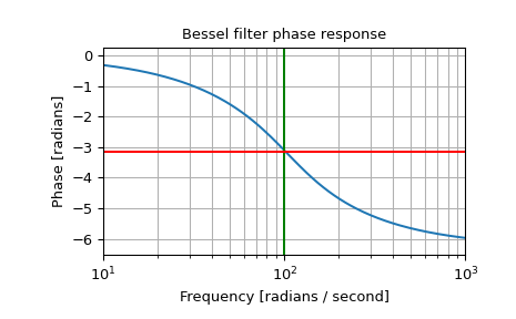
>>> plt.figure() >>> plt.semilogx(w, np.unwrap(np.angle(h))) >>> plt.axvline(100, color='green') # cutoff frequency >>> plt.axhline(-np.pi, color='red') # phase midpoint >>> plt.title('Bessel filter phase response') >>> plt.xlabel('Frequency [radians / second]') >>> plt.ylabel('Phase [radians]') >>> plt.margins(0, 0.1) >>> plt.grid(which='both', axis='both') >>> plt.show()
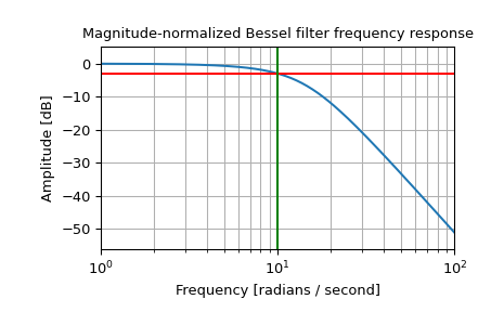
Plot the magnitude-normalized frequency response, showing the -3 dB cutoff:
>>> b, a = signal.bessel(3, 10, 'low', analog=True, norm='mag') >>> w, h = signal.freqs(b, a) >>> plt.semilogx(w, 20 * np.log10(np.abs(h))) >>> plt.axhline(-3, color='red') # -3 dB magnitude >>> plt.axvline(10, color='green') # cutoff frequency >>> plt.title('Magnitude-normalized Bessel filter frequency response') >>> plt.xlabel('Frequency [radians / second]') >>> plt.ylabel('Amplitude [dB]') >>> plt.margins(0, 0.1) >>> plt.grid(which='both', axis='both') >>> plt.show()
Plot the delay-normalized filter, showing the maximally-flat group delay at 0.1 seconds:
>>> b, a = signal.bessel(5, 1/0.1, 'low', analog=True, norm='delay') >>> w, h = signal.freqs(b, a) >>> plt.figure() >>> plt.semilogx(w[1:], -np.diff(np.unwrap(np.angle(h)))/np.diff(w)) >>> plt.axhline(0.1, color='red') # 0.1 seconds group delay >>> plt.title('Bessel filter group delay') >>> plt.xlabel('Frequency [radians / second]') >>> plt.ylabel('Group delay [seconds]') >>> plt.margins(0, 0.1) >>> plt.grid(which='both', axis='both') >>> plt.show()