sklearn.metrics .roc_curve
Note: this implementation is restricted to the binary classification task.
Parameters : y_true array-like of shape (n_samples,)
True binary labels. If labels are not either or , then pos_label should be explicitly given.
y_score array-like of shape (n_samples,)
Target scores, can either be probability estimates of the positive class, confidence values, or non-thresholded measure of decisions (as returned by “decision_function” on some classifiers).
pos_label int, float, bool or str, default=None
The label of the positive class. When pos_label=None , if y_true is in or , pos_label is set to 1, otherwise an error will be raised.
sample_weight array-like of shape (n_samples,), default=None
drop_intermediate bool, default=True
Whether to drop some suboptimal thresholds which would not appear on a plotted ROC curve. This is useful in order to create lighter ROC curves.
New in version 0.17: parameter drop_intermediate.
Increasing false positive rates such that element i is the false positive rate of predictions with score >= thresholds[i] .
tpr ndarray of shape (>2,)
Increasing true positive rates such that element i is the true positive rate of predictions with score >= thresholds[i] .
thresholds ndarray of shape (n_thresholds,)
Decreasing thresholds on the decision function used to compute fpr and tpr. thresholds[0] represents no instances being predicted and is arbitrarily set to np.inf .
Plot Receiver Operating Characteristic (ROC) curve given an estimator and some data.
Plot Receiver Operating Characteristic (ROC) curve given the true and predicted values.
Compute error rates for different probability thresholds.
Compute the area under the ROC curve.
Since the thresholds are sorted from low to high values, they are reversed upon returning them to ensure they correspond to both fpr and tpr , which are sorted in reversed order during their calculation.
An arbitrary threshold is added for the case tpr=0 and fpr=0 to ensure that the curve starts at (0, 0) . This threshold corresponds to the np.inf .
Fawcett T. An introduction to ROC analysis[J]. Pattern Recognition Letters, 2006, 27(8):861-874.
>>> import numpy as np >>> from sklearn import metrics >>> y = np.array([1, 1, 2, 2]) >>> scores = np.array([0.1, 0.4, 0.35, 0.8]) >>> fpr, tpr, thresholds = metrics.roc_curve(y, scores, pos_label=2) >>> fpr array([0. , 0. , 0.5, 0.5, 1. ]) >>> tpr array([0. , 0.5, 0.5, 1. , 1. ]) >>> thresholds array([ inf, 0.8 , 0.4 , 0.35, 0.1 ])
sklearn.metrics .RocCurveDisplay
It is recommend to use from_estimator or from_predictions to create a RocCurveDisplay . All parameters are stored as attributes.
Parameters : fpr ndarray
tpr ndarray
roc_auc float, default=None
Area under ROC curve. If None, the roc_auc score is not shown.
estimator_name str, default=None
Name of estimator. If None, the estimator name is not shown.
pos_label int, float, bool or str, default=None
The class considered as the positive class when computing the roc auc metrics. By default, estimators.classes_[1] is considered as the positive class.
chance_level_ matplotlib Artist or None
The chance level line. It is None if the chance level is not plotted.
figure_ matplotlib Figure
Figure containing the curve.
Compute Receiver operating characteristic (ROC) curve.
Plot Receiver Operating Characteristic (ROC) curve given an estimator and some data.
Plot Receiver Operating Characteristic (ROC) curve given the true and predicted values.
Compute the area under the ROC curve.
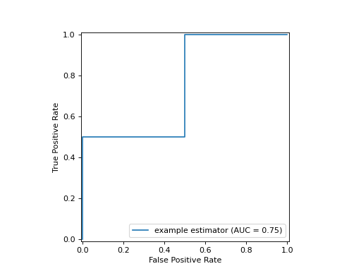
>>> import matplotlib.pyplot as plt >>> import numpy as np >>> from sklearn import metrics >>> y = np.array([0, 0, 1, 1]) >>> pred = np.array([0.1, 0.4, 0.35, 0.8]) >>> fpr, tpr, thresholds = metrics.roc_curve(y, pred) >>> roc_auc = metrics.auc(fpr, tpr) >>> display = metrics.RocCurveDisplay(fpr=fpr, tpr=tpr, roc_auc=roc_auc, . estimator_name='example estimator') >>> display.plot() >>> plt.show()
Create a ROC Curve display from an estimator.
Plot ROC curve given the true and predicted values.
plot ([ax, name, plot_chance_level, . ])
Create a ROC Curve display from an estimator.
Parameters : estimator estimator instance
Fitted classifier or a fitted Pipeline in which the last estimator is a classifier.
X of shape (n_samples, n_features)
y array-like of shape (n_samples,)
sample_weight array-like of shape (n_samples,), default=None
drop_intermediate bool, default=True
Whether to drop some suboptimal thresholds which would not appear on a plotted ROC curve. This is useful in order to create lighter ROC curves.
Specifies whether to use predict_proba or decision_function as the target response. If set to ‘auto’, predict_proba is tried first and if it does not exist decision_function is tried next.
pos_label int, float, bool or str, default=None
The class considered as the positive class when computing the roc auc metrics. By default, estimators.classes_[1] is considered as the positive class.
name str, default=None
Name of ROC Curve for labeling. If None , use the name of the estimator.
ax matplotlib axes, default=None
Axes object to plot on. If None , a new figure and axes is created.
plot_chance_level bool, default=False
Whether to plot the chance level.
Keyword arguments to be passed to matplotlib’s plot for rendering the chance level line.
Keyword arguments to be passed to matplotlib’s plot .
Returns : display RocCurveDisplay
Compute Receiver operating characteristic (ROC) curve.
ROC Curve visualization given the probabilities of scores of a classifier.
Compute the area under the ROC curve.
>>> import matplotlib.pyplot as plt >>> from sklearn.datasets import make_classification >>> from sklearn.metrics import RocCurveDisplay >>> from sklearn.model_selection import train_test_split >>> from sklearn.svm import SVC >>> X, y = make_classification(random_state=0) >>> X_train, X_test, y_train, y_test = train_test_split( . X, y, random_state=0) >>> clf = SVC(random_state=0).fit(X_train, y_train) >>> RocCurveDisplay.from_estimator( . clf, X_test, y_test) >>> plt.show()
classmethod from_predictions ( y_true , y_pred , * , sample_weight = None , drop_intermediate = True , pos_label = None , name = None , ax = None , plot_chance_level = False , chance_level_kw = None , ** kwargs ) [source] 
Plot ROC curve given the true and predicted values.
y_pred array-like of shape (n_samples,)
Target scores, can either be probability estimates of the positive class, confidence values, or non-thresholded measure of decisions (as returned by “decision_function” on some classifiers).
sample_weight array-like of shape (n_samples,), default=None
drop_intermediate bool, default=True
Whether to drop some suboptimal thresholds which would not appear on a plotted ROC curve. This is useful in order to create lighter ROC curves.
pos_label int, float, bool or str, default=None
The label of the positive class. When pos_label=None , if y_true is in or , pos_label is set to 1, otherwise an error will be raised.
name str, default=None
Name of ROC curve for labeling. If None , name will be set to «Classifier» .
ax matplotlib axes, default=None
Axes object to plot on. If None , a new figure and axes is created.
plot_chance_level bool, default=False
Whether to plot the chance level.
Keyword arguments to be passed to matplotlib’s plot for rendering the chance level line.
Additional keywords arguments passed to matplotlib plot function.
Returns : display RocCurveDisplay
Object that stores computed values.
Compute Receiver operating characteristic (ROC) curve.
ROC Curve visualization given an estimator and some data.
Compute the area under the ROC curve.
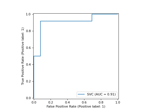
>>> import matplotlib.pyplot as plt >>> from sklearn.datasets import make_classification >>> from sklearn.metrics import RocCurveDisplay >>> from sklearn.model_selection import train_test_split >>> from sklearn.svm import SVC >>> X, y = make_classification(random_state=0) >>> X_train, X_test, y_train, y_test = train_test_split( . X, y, random_state=0) >>> clf = SVC(random_state=0).fit(X_train, y_train) >>> y_pred = clf.decision_function(X_test) >>> RocCurveDisplay.from_predictions( . y_test, y_pred) >>> plt.show()

plot ( ax = None , * , name = None , plot_chance_level = False , chance_level_kw = None , ** kwargs ) [source] 
Extra keyword arguments will be passed to matplotlib’s plot .
Parameters : ax matplotlib axes, default=None
Axes object to plot on. If None , a new figure and axes is created.
name str, default=None
Name of ROC Curve for labeling. If None , use estimator_name if not None , otherwise no labeling is shown.
plot_chance_level bool, default=False
Whether to plot the chance level.
Keyword arguments to be passed to matplotlib’s plot for rendering the chance level line.
Keyword arguments to be passed to matplotlib’s plot .
Returns : display RocCurveDisplay
Object that stores computed values.
Как построить кривую ROC в Python (шаг за шагом)

Логистическая регрессия — это статистический метод, который мы используем для подбора модели регрессии, когда переменная отклика является бинарной. Чтобы оценить, насколько хорошо модель логистической регрессии соответствует набору данных, мы можем взглянуть на следующие две метрики:
- Чувствительность: вероятность того, что модель предсказывает положительный результат для наблюдения, когда результат действительно положительный. Это также называется «истинно положительным показателем».
- Специфичность: вероятность того, что модель предсказывает отрицательный результат для наблюдения, когда результат действительно отрицательный. Это также называется «истинной отрицательной ставкой».
Один из способов визуализировать эти две метрики — создать кривую ROC , которая означает кривую «рабочей характеристики приемника». Это график, отображающий чувствительность и специфичность модели логистической регрессии.
В следующем пошаговом примере показано, как создать и интерпретировать кривую ROC в Python.
Шаг 1: Импортируйте необходимые пакеты
Во-первых, мы импортируем пакеты, необходимые для выполнения логистической регрессии в Python:
import pandas as pd import numpy as np from sklearn. model_selection import train_test_split from sklearn. linear_model import LogisticRegression from sklearn import metrics import matplotlib.pyplot as plt Шаг 2: Подберите модель логистической регрессии
Далее мы импортируем набор данных и подгоним к нему модель логистической регрессии:
#import dataset from CSV file on Github url = "https://raw.githubusercontent.com/Statology/Python-Guides/main/default.csv" data = pd.read_csv (url) #define the predictor variables and the response variable X = data[['student', 'balance', 'income']] y = data['default'] #split the dataset into training (70%) and testing (30%) sets X_train,X_test,y_train,y_test = train_test_split(X,y,test_size=0.3,random_state=0) #instantiate the model log_regression = LogisticRegression() #fit the model using the training data log_regression. fit (X_train,y_train) Шаг 3: Постройте кривую ROC
Далее мы рассчитаем долю истинных положительных и ложных положительных результатов и создадим кривую ROC с помощью пакета визуализации данных Matplotlib:
#define metrics y_pred_proba = log_regression. predict_proba (X_test)[. 1] fpr, tpr, _ = metrics. roc_curve (y_test, y_pred_proba) #create ROC curve plt.plot (fpr,tpr) plt.ylabel('True Positive Rate') plt.xlabel('False Positive Rate') plt.show() 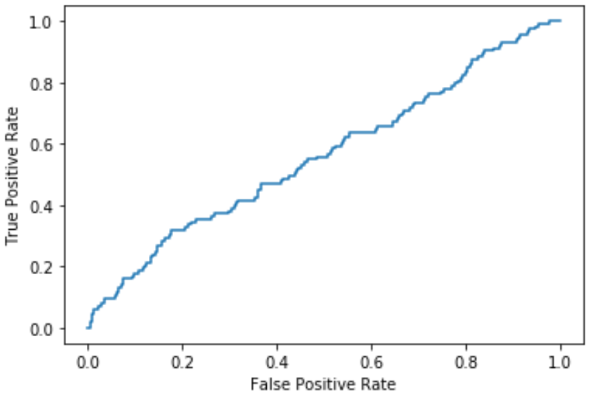
Чем больше кривая охватывает верхний левый угол графика, тем лучше модель классифицирует данные по категориям.
Как видно из графика выше, эта модель логистической регрессии довольно плохо справляется с классификацией данных по категориям.
Чтобы дать количественную оценку, мы можем рассчитать AUC — площадь под кривой, которая говорит нам, какая часть графика расположена под кривой.
Чем ближе AUC к 1, тем лучше модель. Модель со значением AUC, равным 0,5, ничем не лучше модели со случайными классификациями.
Шаг 4: Рассчитайте AUC
Мы можем использовать следующий код для расчета AUC модели и отображения его в правом нижнем углу графика ROC:
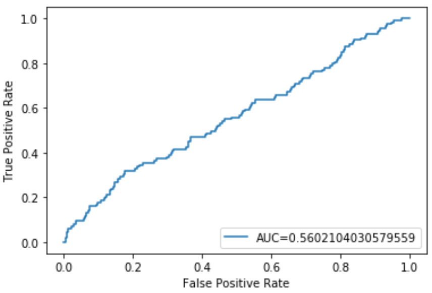
#define metrics y_pred_proba = log_regression. predict_proba (X_test)[. 1] fpr, tpr, _ = metrics. roc_curve (y_test, y_pred_proba) auc = metrics. roc_auc_score (y_test, y_pred_proba) #create ROC curve plt.plot (fpr,tpr,label=» AUC kg-card kg-image-card»>
AUC для этой модели логистической регрессии оказывается равным 0,5602.Поскольку это близко к 0,5, это подтверждает, что модель плохо справляется с классификацией данных.